• Getting an idea of how clustering works, and comparing it to alternative, existing classification techniques
• Using scikit-learn and matplotlib to enrich the possibilities of dataset choices, and to get a professional-looking graphical representation of the data
• Implementing the k-means clustering algorithm
• Implementing the nearest neighbor method, and comparing the results with that of the k-means

In this chapter we will be reviewing two cases of unsupervised learning.

Unsupervised learning basically consists of finding patterns on a previous dataset. Normally, little or no information is given for this technique and the procedure should be able to automatically determine how the information is organized, and recognize the different structures in the data organization.

k-means tries to divide a set of samples in k disjoint groups or clusters using the mean value of the members as the main indicator. This point is normally called a Centroid, referring to the arithmetical entity with the same name, and is represented as a vector in a space of arbitrary dimensions.

k-means is a naive method because it works by looking for the appropriate centroids but doesn't know a priori what the number of clusters is.

In order to get an evaluation of how many clusters give a good representation of the provided data, one of the more popular methods is the Elbow method.

Algorithm iteration criterion

The criterion and goal of this method is to minimize the sum of squared distances from the cluster's member to the actual centroid of all cluster-contained samples. This is also known as Minimization of Inertia.

Error Minimization criteria for k-means

Latex: \sum_{i=0}^{n}\lim_{\mu_j\epsilon C}(\left \| x_{j} - \mu_i \right \|^{2}).

The mechanism of the k-means algorithm can be summarized by the following flowchart:

Simplified flowchart of the k-means process

The algorithm can be simplified as follows:

The stopping conditions could be of various types:

k-means simplified graphic

k-nn can be implemented in more than one of our configurations, but in this chapter we will use the Semi Supervised approach. We will start from a certain number of already assigned samples, and we will later guess the cluster membership based on the characteristics of the train set.

Nearest neighbor algorithm

In the previous figure, we can see a breakdown of the algorithm. It can be summarized by the following steps:

We will discuss some useful libraries in the following sections.

matplotlib plotting library

Data plotting is an integral part of data science discipline. For this reason, we need a very powerful framework to be able to plot our results. For this task, we do not have a general solution implemented in TensorFlow, we will use the matplotlib library.

From the matplotlib site (http://matplotlib.org/), the definition is:

"matplotlib is a Python 2D plotting library which produces publication quality figures in a variety of hardcopy formats and interactive environments across platforms."

Sample synthetic data plotting

In this example, we will generate a list of 100 random numbers, generate a plot of the samples, and save the results in a graphics file:

    import tensorflow as tf
    import numpy as np
    import matplotlib.pyplot as plt
    with tf.Session() as sess:
        fig, ax = plt.subplots()
        ax.plot(tf.random_normal([100]).eval(), tf.random_normal([100] ).eval(),'o')
        ax.set_title('Sample random plot for TensorFlow')
        plt.savefig("result.png")

This is the resulting image:

Sample plot generated with TensorFlow and matplotlib

Tip

In order to see a more general explanation of the scikit dataset module, please refer to: http://matplotlib.org/.

Synthetic dataset types

Some of the generated dataset types we'll be using are:

Blob, circle, and moon dataset types

sklearn.datasets.make_blobs(n_samples=100, n_features=2,  centers=3, cluster_std=1.0, center_box=(-10.0, 10.0),  shuffle=True, random_state=None) 

sklearn.datasets.make_circles(n_samples=100,shuffle=True,noise=None, random_state=None,factor=0.8) 

During this chapter, we'll be using generated datasets that are specially crafted to have special properties. Two of the target properties are the possibility of linear separation of classes and the existence of clearly separated clusters (or not).

centers = [(-2, -2), (-2, 1.5), (1.5, -2), (2, 1.5)] 
data, features = make_blobs (n_samples=200, centers=centers, n_features = 2, cluster_std=0.8, shuffle=False, random_state=42) 

    ax.scatter(np.asarray(centers).transpose()[0], np.asarray(centers).transpose()[1], marker = 'o', s = 250)
    plt.plot()

The points variable contains the 2D coordinates of the dataset points, the centroids variable will contain the coordinates of the center points of the groups, and the cluster_assignments variable contains the centroid index for each data element.

For example, cluster_assignments[2] = 1 indicates that the data[2] data point pertains to the cluster with the center, centroid 1. The location of centroid 1 is located in centroids[1].

points=tf.Variable(data) 
cluster_assignments = tf.Variable(tf.zeros([N], dtype=tf.int64)) 
centroids = tf.Variable(tf.slice(points.initialized_value(), [0,0], [K,2])) 

Then we can draw the position of these centroids using matplotlib:

fig, ax = plt.subplots() 
ax.scatter(np.asarray(centers).transpose()[0], np.asarray(centers).transpose()[1], marker = 'o', s = 250) 
plt.show() 

Initial center seeding

Then we will do N copies of all centroids, K copies of each point, and N x K copies of every point so we can calculate the distances between each point and every centroid, for each dimension:

rep_centroids = tf.reshape(tf.tile(centroids, [N, 1]), [N, K, 2]) 
rep_points = tf.reshape(tf.tile(points, [1, K]), [N, K, 2]) 
sum_squares = tf.reduce_sum(tf.square(rep_points - rep_centroids),  
reduction_indices=2) 

Then we perform the sum for all dimensions and get the index of the lowest sum (this will be the index of the centroid or cluster assigned for each point):

best_centroids = tf.argmin(sum_squares, 1) 

Centroids will also be updated with a bucket:mean function, defined in the full source code.

This is the stop condition that the new centroids and assignments don't change:

did_assignments_change = tf.reduce_any(tf.not_equal(best_centroids, cluster_assignments)) 

Here, we use control_dependencies to calculate whether we need to update the centroids:

with tf.control_dependencies([did_assignments_change]): 
    do_updates = tf.group( 
    centroids.assign(means), 
    cluster_assignments.assign(best_centroids)) 

We get the following output when the program is executed:

This is a summarizing graphic of the centroid changes after a round of iterations with the original clusters drawn as they were generated from the algorithm.

In the following image, we represent the different stages in the application of the k-means algorithm for this clearly separated case:

Centroid changes per iteration

Following is the complete source code:

import tensorflow as tf 
import numpy as np 
import time 
 
import matplotlib 
import matplotlib.pyplot as plt 
 
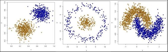
from sklearn.datasets.samples_generator import make_blobs 
from sklearn.datasets.samples_generator import make_circles 
 
DATA_TYPE = 'blobs' 
 
# Number of clusters, if we choose circles, only 2 will be enough 
if (DATA_TYPE == 'circle'): 
    K=2 
else: 
    K=4 
 
# Maximum number of iterations, if the conditions are not met 
MAX_ITERS = 1000 
 
start = time.time() 
 
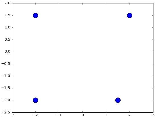
centers = [(-2, -2), (-2, 1.5), (1.5, -2), (2, 1.5)] 
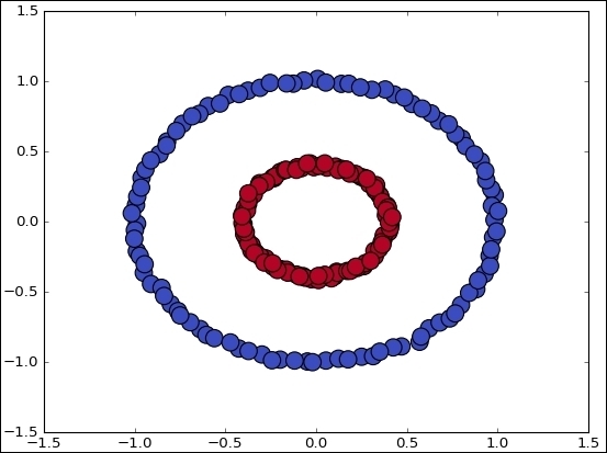
if (DATA_TYPE == 'circle'): 
    data, features = make_circles(n_samples=200, shuffle=True, noise= 0.01, factor=0.4) 
else: 
    data, features = make_blobs (n_samples=200, centers=centers, n_features = 2, cluster_std=0.8, shuffle=False, random_state=42) 
 
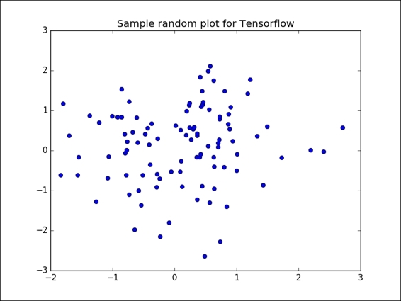
fig, ax = plt.subplots() 
ax.scatter(np.asarray(centers).transpose()[0], np.asarray(centers).transpose()[1], marker = 'o', s = 250) 
plt.show() 
 
fig, ax = plt.subplots() 
if (DATA_TYPE == 'blobs'): 
ax.scatter(np.asarray(centers).transpose()[0], np.asarray(centers).transpose()[1], marker = 'o', s = 250) 
ax.scatter(data.transpose()[0], data.transpose()[1], marker = 'o', s = 100, c = features, cmap=plt.cm.coolwarm ) 
plt.plot() 
 
points=tf.Variable(data) 
cluster_assignments = tf.Variable(tf.zeros([N], dtype=tf.int64)) 
centroids = tf.Variable(tf.slice(points.initialized_value(), [0,0], [K,2])) 
 
sess = tf.Session() 
sess.run(tf.initialize_all_variables()) 
 
rep_centroids = tf.reshape(tf.tile(centroids, [N, 1]), [N, K, 2]) 
rep_points = tf.reshape(tf.tile(points, [1, K]), [N, K, 2]) 
sum_squares = tf.reduce_sum(tf.square(rep_points - rep_centroids),  
reduction_indices=2) 
best_centroids = tf.argmin(sum_squares, 1) 
 
did_assignments_change = tf.reduce_any(tf.not_equal(best_centroids, cluster_assignments)) 
 
def bucket_mean(data, bucket_ids, num_buckets): 
total = tf.unsorted_segment_sum(data, bucket_ids, num_buckets) 
count = tf.unsorted_segment_sum(tf.ones_like(data), bucket_ids, num_buckets) 
return total / count 
 
means = bucket_mean(points, best_centroids, K) 
 
with tf.control_dependencies([did_assignments_change]): 
do_updates = tf.group( 
centroids.assign(means), 
cluster_assignments.assign(best_centroids)) 
 
changed = True 
iters = 0 
 
fig, ax = plt.subplots() 
if (DATA_TYPE == 'blobs'): 
    colourindexes=[2,1,4,3] 
else: 
    colourindexes=[2,1] 
while changed and iters < MAX_ITERS: 
fig, ax = plt.subplots() 
iters += 1 
[changed, _] = sess.run([did_assignments_change, do_updates]) 
[centers, assignments] = sess.run([centroids, cluster_assignments]) 
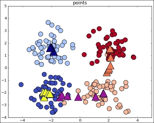
ax.scatter(sess.run(points).transpose()[0], sess.run(points).transpose()[1], marker = 'o', s = 200, c = assignments, cmap=plt.cm.coolwarm ) 
ax.scatter(centers[:,0],centers[:,1], marker = '^', s = 550, c = colourindexes, cmap=plt.cm.plasma) 
ax.set_title('Iteration ' + str(iters)) 
plt.savefig("kmeans" + str(iters) +".png") 
 
ax.scatter(sess.run(points).transpose()[0], sess.run(points).transpose()[1], marker = 'o', s = 200, c = assignments, cmap=plt.cm.coolwarm ) 
plt.show() 
 
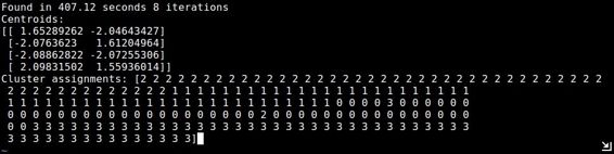
end = time.time() 
print ("Found in %.2f seconds" % (end-start)), iters, "iterations" 
print "Centroids:" 
print centers 
print "Cluster assignments:", assignments 

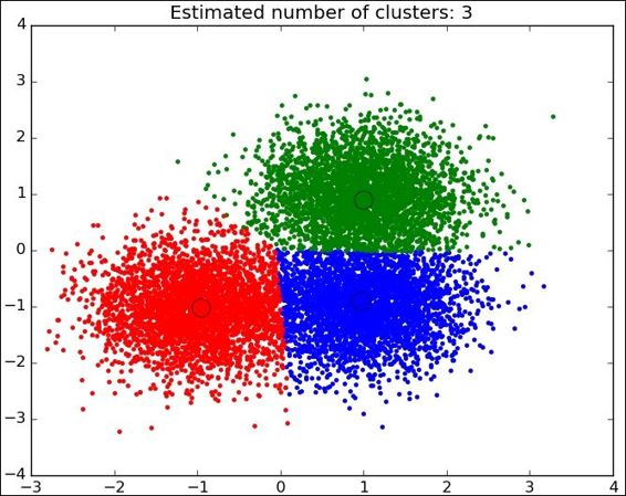
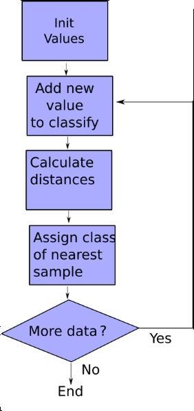
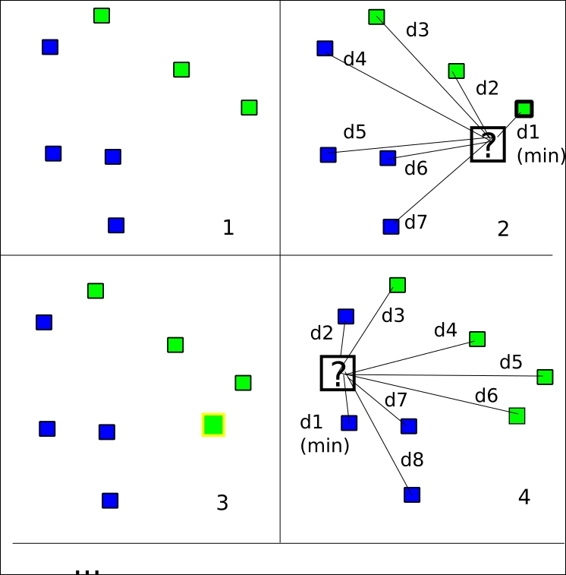
This is the simplest case for observing the algorithm mechanics. When the data comes from the real world, the classes are normally not so clearly separated and it is more difficult to label the data samples.

For the circular plot, we observe that this data characterization is not simple to represent by a simple set of means. As the image clearly shows, the two circles either share a Centroid position, or are really close and so we cannot predict a clear outcome:

Circle type dataset

For this dataset, we are only using two classes to be sure the main drawbacks of this algorithm are understood:

k-means applied to a circular synthetic dataset

As we can see, the initial centers drifted toward the areas that had the most concentrated sample numbers, and so divided the data linearly. This is one of the limitations of the simple models we are employing at this stage. To cope with nonlinear separability samples, we can try other statistical approaches outside the scope of this chapter, such as density-based spatial clustering of applications with noise (DBSCAN).

The dataset is the same circular classes dataset from the first example with two classes, but this time we will increase the error probability by adding a bit more noise (from 0.01 to 0.12):

data, features = make_circles(n_samples=N, shuffle=True, noise=0.12,factor=0.4)

This is the resulting training data plot:

The variables that will sustain data are simply the original data and a test list, which will hold the calculated classes for the test data:

data, features = make_circles(n_samples=N, shuffle=True, noise= 0.12, factor=0.4)
tr_data, tr_features= data[:cut], features[:cut]
te_data,te_features=data[cut:], features[cut:]
test=[]

In clustering, we will use the function to optimize as the Euclidean distance, the same as Chapter 1, Exploring and Transforming Data. It is calculated on the cluster assignment loop, getting the distance from the new point to the existing training points, asking for the index of the minimum, and then using that index to search the class of the nearest neighbor:

distances = tf.reduce_sum(tf.square(tf.sub(i , tr_data)),reduction_indices=1)
neighbor = tf.arg_min(distances,0)

In this simple example, we will finish once all the elements of the test partition have been visited.

Here is a graphic of the test data class assignation where we can see the clearly separated classes. We can observe that, at least with this limited dataset scope, this method works better than the non-overlapping, blob-optimizing, k-means method.

Following is the complete source code:

import tensorflow as tf 
import numpy as np 
import time 
 
import matplotlib 
import matplotlib.pyplot as plt 
 
from sklearn.datasets.samples_generator import make_circles 
 
N=210 
K=2 
# Maximum number of iterations, if the conditions are not met 
MAX_ITERS = 1000 
cut=int(N*0.7) 
 
start = time.time() 
 
data, features = make_circles(n_samples=N, shuffle=True, noise= 0.12, factor=0.4) 
tr_data, tr_features= data[:cut], features[:cut] 
te_data,te_features=data[cut:], features[cut:] 
test=[] 
 
fig, ax = plt.subplots() 
ax.scatter(tr_data.transpose()[0], tr_data.transpose()[1], marker = 'o', s = 100, c = tr_features, cmap=plt.cm.coolwarm ) 
plt.plot() 
 
sess = tf.Session() 
sess.run(tf.initialize_all_variables()) 
 
for i, j in zip(te_data, te_features): 
    distances = tf.reduce_sum(tf.square(tf.sub(i , tr_data)),reduction_indices=1) 
    neighbor = tf.arg_min(distances,0) 
 
    test.append(tr_features[sess.run(neighbor)]) 
print test 
fig, ax = plt.subplots() 
ax.scatter(te_data.transpose()[0], te_data.transpose()[1], marker = 'o', s = 100, c = test, cmap=plt.cm.coolwarm ) 
plt.plot() 
 
end = time.time() 
print ("Found in %.2f seconds" % (end-start)) 
 
print "Cluster assignments:", test