In the previous chapter, we have seen an approach to model a part of reality as a linear function, which has independent variables and bias minimized an error function.
This particular analysis is not enough except for some very clearly defined problems, with expected results being continuous variables and function.
But what would happen if we are faced with data with qualitative dependent variables? For example, the presence or absence of a determinate feature; has a subject got blond hair? Has the patient had a previous illness?
These are the kinds of problem that we will be working on in this chapter.
The kind of problem that linear regression aims to solve is not the prediction of a value based on a continuous function, this time we want to know the probability for a sample of pertaining to a determined class.
In this chapter, we will rely on a generalization of the linear model solving a regression, but with the final objective of solving classification problems where we have to apply tags or assign all the elements from an observation set to predefined groups.
In the preceding figure, we can see how the old and new problems can be classified. The first one (linear regression) can be imagined as a continuum of increasingly growing values.
The other is a domain where the output can have just two different values, based on the x value. In the particular case of the second graphic, we can see a particular bias to one of the options, toward the extremes: on the left there is a bias towards the 0 y value, and to the right the bias is towards a value of 1.
This terminology can be bit tricky given that even when we are doing a regression, thus looking for a continuous value, in reality, the final objective is building a prediction for a classification problem, with discrete variables.
The key here is to understand that we will obtain probabilities of an item pertaining to a class, and not a totally discrete value.
Before we study the logistic function, we will review the original function on which it is based, and which gives it some of its more general properties.
Essentially, when we talk about the logit
function, we are working with the function of a random variable p, more specifically, one corresponding with a Bernoulli distribution.
Before explaining theoretical details it is worthwhile noting that a Bernoulli distribution is a random variable that:
It can be expressed as follows (for a random variable X with Bernoulli distribution):
This is the kind of probability distribution that will represent the probability of occurrence of the events as binary options, just as we want to represent our variables (existence of features, event occurrence, causality of phenomena, and so on).
As we are trying to build a generalized linear model, we want to start from a linear function, and from the dependent variable, obtain a mapping to a probability distribution.
Since the options are of a binary nature, the normally chosen distribution is the recently mentioned Bernoulli distribution, and the link function, leaning toward the logistic function, is the logit
function.
One of the possible variables that we could utilize, is the natural logarithm of the odds that p equals one. This function is called the logit
function:
We can also call the logit
function a log-odd function, because we are calculating the log of the odds (p/1-p) for a given probability p:
So, as we can visually infer, replacing X with the combination of the independent variables, no matter the value of them, replacing X with any occurrence from minus infinity to infinity, we are scaling the response to be within 0 and 1.
The logistic function will serve us to represent the binary options in our new regression tasks.
In the following figure, you will find the graphical representation of the sigmoid
function:
Graphical representation of the logistic function or Sigmoid
The logistic function δ(t) is defined as follows:
The normal interpretation of this equation is that t represents a simple independent variable. But we will improve this model, and will assume that t is a linear function of a single explanatory variable x (the case where t is a linear combination of multiple explanatory variables is treated similarly).
We will then express t as the following:
So we start from the following equation:
With all these elements, we can calculate the regression equation, which will give us the regressed probability:
The following graphic will show how the mapping from arbitrary range will be finally transformed to range [0, 1], which can be interpreted as probability p of the occurrence of the event being represented:
What effects will make changes to the parameters of the linear function? They are the values that will change the central slope and the displacement from zero of the sigmoid
function, allowing it to more exactly reduce the error between the regressed values and the real data points.
Every curve in the function space can be described by the possible objectives it could be applied to. In the case of the logistic function, they are:
In the previous section we saw our approximated [latex]\hat p[/latex] function, which will model the probability of a sample being of a particular class. In order to measure how well we are approximating to the solution, we will look for a carefully chosen loss function.
This loss function is expressed as:
The main property of this loss function is that it doesn't penalize the error in a similar manner, the error penalization factor grows asymptotically when the error increases far beyond 0.5.
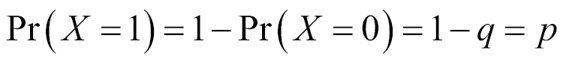
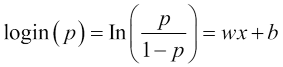
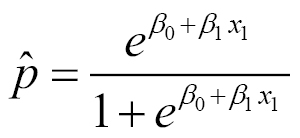
Up until now, we have been classifying for the case of only two classes, or in probabilistic language, event occurrence probabilities, p.
In the case of having more than two classes to decide from, there are two main approaches; one versus one, and one versus all.
softmax
regression, a generalization of the logistic regression for n classes.So we will be changing, for training samples, from binary labels ( y(i)ε{0,1}), to vector labels, using the handle y(i)ε{1,...,K}, where K is the number of classes, and the label Y can take on K different values, rather than only two.
So for this particular technique, given a test input X, we want to estimate the probability that P(y=k|x) for each value of k=1,...,K. The softmax
regression will output a K-dimensional vector (whose elements sum to 1), giving us our K estimated probabilities.
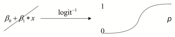
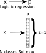
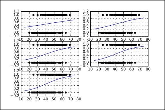
In the following diagram, we represent the mapping that occurs on the probability mappings of the uniclass and multiclass logistic regression:
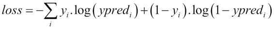
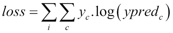
The cost function of the softmax
function is an adapted cross entropy function, which is not linear, and thus penalizes the big order function differences much more than the very small ones.
Here, c is the class number and I the individual train sample index, and yc is 1 for the expected class and 0 for the rest.
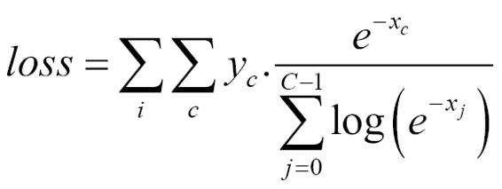
Expanding this equation, we get the following:
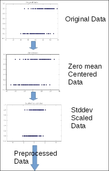
As we will see in the following sections, for logistic regression we will be using the gradient descent
method for minimizing a cost function.
This method is very sensitive to the form and the distribution of the feature data.
For this reason, we will be doing some preprocessing in order to get better and faster converging results.
We will leave the theoretical reasons for this method to other books, but we will summarize the reason saying that with normalization, we are smoothing the error surface, allowing the iterative gradient descent
to reach the minimum error faster.
In order to use the softmax
function as the regression function, we must use a type of encoding known as one hot. This form of encoding simply transforms the numerical integer value of a variable into an array, where a list of values is transformed into a list of arrays, each with a length of as many elements as the maximum value of the list, and the value of each elements is represented by adding a one on the index of the value, and leaving the others at zero.
For example, this will be the representation of the list [1, 3, 2, 4] in one hot encoding:
[[0 1 0 0 0] [0 0 0 1 0] [0 0 1 0 0] [0 0 0 0 1]]
In this first example, we will work approximating the probability of the presence of heart disease, using an univariate logistic regression, being this variable, the patients age.
Since version 0.8, TensorFlow has provided a means of generating one hot. The function used for this generation is tf.one_hot
, which has this form:
tf.one_hot(indices, depth, on_value=1, off_value=0, axis=None, dtype=tf.float32, name=None)
This functions generates a generalized one hot encoding data structure, which can specify the values, axis of generation, data type, and so on.
In the resulting tensors, the indicated values of the indexes will take the on_value
, default 1
, and the others will have off_value
, default 0
.
Dtype
is the data type of the generated tensor; the default is float32
.
The depth variable defines how many columns each element will have. We suppose it logically should be max(indices) + 1
, but it could be also cut.
The included method for applying softmax
regression in TensorFlow is tf.nn.log_softmax, with the following form:
tf.nn.log_softmax(logits, name=None)
Here, the arguments are:
logits
: A tensor must be one of the following types: float32
, float64
2D with shape [batch_size, num_classes]
name
: A name for the operation (optional)This function returns a tensor with the same type and shape as logits
.
The first case we will cover is where we want to fit a logistic regression, measuring only one variable and we only have a binary possible result.
For the first simple example, we will use a very simple and studied dataset, first known for being published in the book; Applied Logistic Regression-Third Edition, David W. Hosmer Jr., Stanley Lemeshow, Rodney X. Sturdivant, by Wiley.
Lists the age
in years (AGE), and presence or absence of evidence of significant Coronary Heart Disease (CHD) for 100 subjects in a hypothetical study of risk factors for heart disease. The table also contains an identifier variable (ID) and an age group variable (AGEGRP). The outcome variable is CHD, which is coded with a value of 0
to indicate that CHD is absent, or 1
to indicate that it is present in the individual. In general, any two values could be used, but we have found it most convenient to use zero and one. We refer to this data set as the CHDAGE data.
The CHDAGE dataset is a two-column CSV file that we will download from an external repository.
In the chapter 1, Exploring and Transforming Data, we used native TensorFlow methods for the reading of the dataset. In this chapter, we will use a complementary and popular library to get the data.
The cause for this new addition is that, given that the dataset only has 100 tuples, it is practical to just have to read it in one line, and also we get simple but powerful analysis methods for free, provided by the pandas
library.
So in the first stage of this project, we will start loading an instance of the CHDAGE dataset, then we will print vital statistics about the data, and then proceed to preprocessing.
After doing some plots of the data, we will build a model composed of the activation function, which will be a softmax
function for special cases where it becomes a standard logistic regression; that is when there are only two classes (existence, or not, of the illness).
First, we import the required libraries, and indicate that all our matplotlib
programs will be included inline (if we are using Jupyter):
>>> import pandas as pd
>>> import numpy as np
>>> %matplotlib inline
>>> import matplotlib.pyplot as plt
Then we read the data and ask pandas
to check important statistical information about the dataset:
>>> df = pd.read_csv("data/CHD.csv", header=0)
>>> print df.describe()
age chd
count 100.000000 100.00000
mean 44.380000 0.43000
std 11.721327 0.49757
min 20.000000 0.00000
25% 34.750000 0.00000
50% 44.000000 0.00000
75% 55.000000 1.00000
max 69.000000 1.000000
We then proceed with drawing the data to get an idea of the data:
plt.figure() # Create a new figure
plt.scatter(df['age'],df['chd']) #Plot a scatter draw of the random datapoints
Here, we describe the sections of the code where we will build the elements of the model, starting from the following variables:
learning_rate = 0.8 #Learning speed batch_size = 100 #number of samples for the batch display_step = 2 #number of steps before showing progress
Here, we create the initial variables and placeholders for the graph, the univariate x
and y
float values:
x = tf.placeholder("float", [None, 1]) # Placeholder for the 1D data y = tf.placeholder("float", [None, 2]) # Placeholder for the classes (2)
Now we will create linear model variables, which will be modified and updated as the model fitting goes on:
W = tf.Variable(tf.zeros([1, 2])) b = tf.Variable(tf.zeros([2]))
And finally, we will build the activation function applying the softmax
operation to the linear function:
activation = tf.nn.softmax(tf.matmul(x, W) + b)
Here, we just define the cross correlation function as the loss
function, and define the optimizer
operation, which will be the gradient descent
. This will be explained in the following chapters; for now, you can see it as a black box that will change the variables until the loss is minimized:
cost = tf.reduce_mean(-tf.reduce_sum(y*tf.log(activation), reduction_indices=1))
optimizer = tf.train.GradientDescentOptimizer(learning_rate).minimize(cost)
#Iterate through all the epochs
for epoch in range(training_epochs):
avg_cost = 0.
total_batch = 400/batch_size
# Loop over all batches
for i in range(total_batch):
# Transform the array into a one hot format
temp=tf.one_hot(indices = df['chd'].values, depth=2, on_value = 1, off_value = 0, axis = -1 , name = "a")
batch_xs, batch_ys =(np.transpose([df['age']])-44.38)/11.721327, temp
# Fit training using batch data
sess.run(optimizer, feed_dict={x: batch_xs.astype(float), y: batch_ys.eval()})
# Compute average loss, suming the corrent cost divided by the batch total number
avg_cost += sess.run(cost, feed_dict={x: batch_xs.astype(float), y: batch_ys.eval()})/total_batch
This will be the output of the program:
Epoch: 0001 cost= 0.638730764
[ 0.04824295 -0.04824295]
[[-0.17459483 0.17459483]]
Epoch: 0002 cost= 0.589489654
[ 0.08091066 -0.08091066]
[[-0.29231569 0.29231566]]
Epoch: 0003 cost= 0.565953553
[ 0.10427245 -0.10427245]
[[-0.37499282 0.37499279]]
Epoch: 0004 cost= 0.553756475
[ 0.12176144 -0.12176143]
[[-0.43521613 0.4352161 ]]
Epoch: 0005 cost= 0.547019333
[ 0.13527818 -0.13527818]
[[-0.48031801 0.48031798]]
Here is the complete source code:
import pandas as pd
import numpy as np
get_ipython().magic(u'matplotlib inline')
import matplotlib.pyplot as plt
import tensorflow as tf
df = pd.read_csv("data/CHD.csv", header=0)
# Parameters
learning_rate = 0.2
training_epochs = 5
batch_size = 100
display_step = 1
sess = tf.Session()
b=np.zeros((100,2))
# tf Graph Input
x = tf.placeholder("float", [None, 1])
y = tf.placeholder("float", [None, 2])
# Create model
# Set model weights
W = tf.Variable(tf.zeros([1, 2]))
b = tf.Variable(tf.zeros([2]))
# Construct model
activation = tf.nn.softmax(tf.matmul(x, W) + b)
# Minimize error using cross entropy
cost = tf.reduce_mean(-tf.reduce_sum(y*tf.log(activation), reduction_indices=1)) # Cross entropy
optimizer = tf.train.GradientDescentOptimizer(learning_rate).minimize(cost) # Gradient Descent
# Initializing the variables
init = tf.initialize_all_variables()
# Launch the graph
with tf.Session() as sess:
tf.train.write_graph(sess.graph, './graphs','graph.pbtxt')
sess.run(init)
writer = tf.train.SummaryWriter('./graphs', sess.graph)
#Initialize the graph structure
graphnumber=321
#Generate a new graph
plt.figure(1)
#Iterate through all the epochs
for epoch in range(training_epochs):
avg_cost = 0.
total_batch = 400/batch_size
# Loop over all batches
for i in range(total_batch):
# Transform the array into a one hot format
temp=tf.one_hot(indices = df['chd'].values, depth=2, on_value = 1, off_value = 0, axis = -1 , name = "a")
batch_xs, batch_ys = (np.transpose([df['age']])-44.38)/11.721327, temp
# Fit training using batch data
sess.run(optimizer, feed_dict={x: batch_xs.astype(float), y: batch_ys.eval()})
# Compute average loss, suming the corrent cost divided by the batch total number
avg_cost += sess.run(cost, feed_dict={x: batch_xs.astype(float), y: batch_ys.eval()})/total_batch
# Display logs per epoch step
if epoch % display_step == 0:
print "Epoch:", '%05d' % (epoch+1), "cost=", "{:.8f}".format(avg_cost)
#Generate a new graph, and add it to the complete graph
trX = np.linspace(-30, 30, 100)
print (b.eval())
print (W.eval())
Wdos=2*W.eval()[0][0]/11.721327
bdos=2*b.eval()[0]
# Generate the probabiliy function
trY = np.exp(-(Wdos*trX)+bdos)/(1+np.exp(-(Wdos*trX)+bdos) )
# Draw the samples and the probability function, whithout the normalization
plt.subplot(graphnumber)
graphnumber=graphnumber+1
#Plot a scatter draw of the random datapoints
plt.scatter((df['age']),df['chd'])
plt.plot(trX+44.38,trY) #Plot a scatter draw of the random datapoints
plt.grid(True)
#Plot the final graph
plt.savefig("test.svg")
Using the TensorBoard utility, we will see the operation chain. Note that in half of the operation graphics we define the main global operation (doftmas), and the gradient operations applied to the remaining terms, which are needed to do the loss
function minimization. This is a theme to be talked about in the following chapters.
In this example, we will explore the univariate examples domain, but this time we will use help from a new library, which eases the model building for us, called skflow
.
In the field of machine learning libraries, there is a great number and variety of alternatives. One of the most well-known is sklearn
, which we talked about in Chapter 2, Clustering.
Very early after the release of TensorFlow, a new contribution library appeared, called skflow
, with the main objective of emulating the interface and workflow of sklearn
, which is much more succinct to work in this TensorFlow session environment.
In the following example, we will repeat the analysis of the previous regression, but using the skflow
interface.
In the example, we will also see how skflow automatically generates a detailed and very organized graph for the regression model, just setting a log directory as a parameter.
Here is the code snippet for my_model
:
def my_model(X, y):
return skflow.models.logistic_regression(X, y)
X1 =a.fit_transform(df['age'].astype(float))
y1 = df['chd'].values
classifier = skflow.TensorFlowEstimator(model_fn=my_model, n_classes=2)
Here we can see a detailed view of the logistic regression stage, with the softmax
classifier:
Here is the complete source code:
import tensorflow.contrib.learn as skflow
from sklearn import datasets, metrics, preprocessing
import numpy as np
import pandas as pd
df = pd.read_csv("data/CHD.csv", header=0)
print df.describe()
def my_model(X, y):
return skflow.models.logistic_regression(X, y)
a = preprocessing.StandardScaler()
X1 =a.fit_transform(df['age'].astype(float))
y1 = df['chd'].values
classifier = skflow.TensorFlowEstimator(model_fn=my_model, n_classes=2)
classifier.fit(X1,y1 , logdir='/tmp/logistic')
score = metrics.accuracy_score(df['chd'].astype(float), classifier.predict(X))
print("Accuracy: %f" % score)
In this chapter, we have learned a new modeling technique, the logistic function, and began with a simple approach to the task of classification.
We also learned a new approach for the reading of text-based data via the pandas
library.
Additionally, we have seen a complementary approach to the classical workflow, working with the skflow
library.
In the next chapter, we will start working with more complex architectures, and enter the field where the TensorFlow library excels: the training, testing, and final implementation of neural networks to solve real-world problems.