Convolutional neural networks are part of many of the most advanced models currently being employed. They are used in numerous fields, but the main application field is in the realm of image classification and feature detection.
The topics we will cover in this chapter are as follows:
The neocognitron is a predecessor to convolutional networks, introduced in a 1980 paper by Prof. Fukushima, and is a self-organizing neural network tolerant to shifts and deformation.
This idea appeared again in 1986 in the book version of the original back propagation paper, and it was also employed in 1988 for temporal signals in speech recognition.
The original design was later reviewed and improved in 1998 with LeCun's paper, gradient-based learning applied to document recognition, which presented the LeNet-5 network, which is able to classify handwritten digits. The model showed increased performance compared with other existing models, especially over several variations of SVM, one of the most performant operations in the year of publication.
Then a generalization of that paper came in 2003, with the paper Hierarchical Neural Networks for Image Interpretation . However, in general, we will be using a close representation of LeCun's LeNet paper architecture.
In order to understand the operations being applied to the information in these kinds of operations, we will start by studying the origin of the convolution function, and then we will explain how this concept is applied to the information.
In order to begin following the historical development of the operation, we will start looking at convolution in the continuous domain.
The original use of this function comes from the eighteenth century and can be expressed, in the original application context, as an operation that blends two functions occurring on time.
Mathematically, it can be defined as follows:
When we try to conceptualize this operation as an algorithm, the preceding equation can be explained in the following steps:
When applying the concept of convolution in the discrete domain, kernels are used quite frequently.
Kernels can be defined as nxm-dimensional matrices, which are normally a few elements long in all dimensions and usually, m = n.
The convolution operation consists of multiplying the corresponding pixels with the kernel, one pixel at a time, and summing the values for the purpose of assigning that value to the central pixel.
The same operation will then be applied, shifting the convolution matrix to the left until all possible pixels are visited.
In the following example, we have an image of many pixels and a kernel of size 3x3, which is particularly common in image processing:
Having reviewed the main characteristics of the convolution operation for continuous and discrete fields, let's now look at the use of this operation in machine learning.
The convolution kernels highlight or hide patterns. Depending on the trained (or in the example, manually set) parameters, we can begin to discover parameters, such as orientation and edges in different dimensions. We may also cover some unwanted details or outliers by means such as blurring kernels.
As LeCun in his fundational paper stated:
"Convolutional networks can be seen as synthesizing their own feature extractor."
This characteristic of convolutional neural networks is the main advantage over previous data processing techniques; we can determine with great flexibility the primary components of a determined dataset and represent further samples as a combination of these basic building blocks.
TensorFlow provides a variety of methods for convolution. The canonical form is applied by the conv2d
operation. Lets have a look at the usage of this operation:
tf.nn.conv2d(input, filter, strides, padding, use_cudnn_on_gpu, data_format, name=None)
The parameters we use are as follows:
input
: This is the original tensor to which the operation will be applied. It has a definite format of four dimensions, and the default dimension order is shown next.[batch, in_height, in_width, in_channels]
: Batch is a dimension that allows you to have a collection of images. This order is called NHWC. The other option is NCWH.For example, a single 100x100 pixel color image will have the following shape:
[1,100,100,3]
filter
: This is a tensor representing a kernel
or filter
. It has a very generic method: [filter_height, filter_width, in_channels, out_channels]
strides
: This is a list of four int
tensor datatypes, which indicate the sliding windows for each dimension.Padding
:This can be SAME
or VALID
. SAME
will try to conserve the initial tensor dimension, but VALID
will allow it to grow in case the output size and padding are computed.use_cudnn_on_gpu
:This indicates whether or not to use the CUDA GPU CNN
library to accelerate calculations.data_format
:This specifies the order in which data is organized (NHWC or NCWH).TensorFlow provides a number of ways of applying convolutions, which are listed as follows:
tf.nn.conv2d_transpose
: This applies the transpose (gradient) of conv2d
and is used in deconvolutional networkstf.nn.conv1d
: This performs 1D convolution, given a 3D input and filter
tensorstf.nn.conv3d
: This performs 3D convolution, given a 5D input and filter
tensorsIn this sample code, we will read a grayscale image in the GIF format, which will generate a three-channel tensor but with the same RGB values per pixel. We will then transform the tensor into a real grayscale matrix, apply a kernel
, and retrieve the results in an output image in the JPEG format.
Note that you can tune the parameter in the kernel
variable to observe the effects of the changes in the image.
The following is the sample code:
import tensorflow as tf #Generate the filename queue, and read the gif files contents filename_queue = tf.train.string_input_producer(tf.train.match_filenames_once("data/test.gif")) reader = tf.WholeFileReader() key, value = reader.read(filename_queue) image=tf.image.decode_gif(value) #Define the kernel parameters kernel=tf.constant( [ [[[-1.]],[[-1.]],[[-1.]]], [[[-1.]],[[8.]],[[-1.]]], [[[-1.]],[[-1.]],[[-1.]]] ] ) #Define the train coordinator coord = tf.train.Coordinator() with tf.Session() as sess: tf.initialize_all_variables().run() threads = tf.train.start_queue_runners(coord=coord) #Get first image image_tensor = tf.image.rgb_to_grayscale(sess.run([image])[0]) #apply convolution, preserving the image size imagen_convoluted_tensor=tf.nn.conv2d(tf.cast(image_tensor, tf.float32),kernel,[1,1,1,1],"SAME") #Prepare to save the convolution option file=open ("blur2.jpeg", "wb+") #Cast to uint8 (0..255), previous scalation, because the convolution could alter the scale of the final image out=tf.image.encode_jpeg(tf.reshape(tf.cast(imagen_convoluted_tensor/tf.reduce_max(imagen_convoluted_tensor)*255.,tf.uint8), tf.shape(imagen_convoluted_tensor.eval()[0]).eval())) file.close() coord.request_stop() coord.join(threads)
In the following figure, you can observe how the changes in the parameters affect the outcome of the image. The first image is the original one.
The filter types are from left to right and top to bottom-blur, bottom Sobel (a kind of filter searching from top to bottom edges), emboss (which highlights the corner edges), and outline (which outlines the exterior limits of the figures).
The subsampling operation is performed in TensorFlow by means of an operation called pool. The idea is to apply a kernel (of varying dimensions ) and extract one of the elements covered by the kernel, the max_pool
and avg_pool
being a few of the most well known, which get only the maximum and the average of the elements for an applied kernel.
In the following figure, you can see the action of applying a 2x2 kernel to a one-channel, 16x16 matrix. It just keeps the maximum value of the internal zone it covers.
The type of pooling operations that can be made are also varied; for example, in LeCun's paper, the operation applied to the original pixels has to multiply them for a trainable parameter and add an additional trainable bias
.
The main purpose of subsampling layers is more or less the same as that of convolutional layers; to reduce the quantity and complexity of information while retaining the most important information elements. They build a compact representation of the underlying information.
Subsampling layers also allow important parts of the information to be translated from a detailed to a simpler representation of the data. By sliding the filter across the image, we translate the detected features to more significant image parts, eventually reaching a 1-pixel image, with the feature represented by that pixel value. Conversely, this property could also produce the model to lose the locality of feature detection.
Subsampling layers are much faster to implement because the elimination criterion for unused data elements is really simple; it just needs a couple of comparisons, in general.
First we will analyze the most commonly used pool
operation, max_pool
. It has the following signature:
tf.nn.max_pool(value, ksize, strides, padding, data_format, name)
This method is similar to conv2d
, and the parameters are as follows:
value
: This is a 4D tensor of float32
elements and shape (batch length, height, width, channels)ksize
: This is a list of ints representing the window size on each dimensionstrides
: This is the step of the moving windows on each dimensiondata_format
: This sets the data dimensionsordering
: NHWC, or NCHWpadding
: VALID
or SAME
tf.nn.avg_pool
: This returns a reduced tensor with the avg of each windowtf.nn.max_pool_with_argmax
: This returns the max_pool
tensor and a tensor with the flattened index of the max_value
tf.nn.avg_pool3d
: This performs an avg_pool
operation with a cubic-like window; the input has an additional depthtf.nn.max_pool3d
: This performs the same function as (...
) but applies the max
operationIn the following sample code, we will take an original:
import tensorflow as tf
#Generate the filename queue, and read the gif files contents
filename_queue = tf.train.string_input_producer(tf.train.match_filenames_once("data/test.gif"))
reader = tf.WholeFileReader()
key, value = reader.read(filename_queue)
image=tf.image.decode_gif(value)
#Define the coordinator
coord = tf.train.Coordinator()
def normalize_and_encode (img_tensor):
image_dimensions = tf.shape(img_tensor.eval()[0]).eval()
return tf.image.encode_jpeg(tf.reshape(tf.cast(img_tensor, tf.uint8), image_dimensions))
with tf.Session() as sess:
maxfile=open ("maxpool.jpeg", "wb+")
avgfile=open ("avgpool.jpeg", "wb+")
tf.initialize_all_variables().run()
threads = tf.train.start_queue_runners(coord=coord)
image_tensor = tf.image.rgb_to_grayscale(sess.run([image])[0])
maxed_tensor=tf.nn.avg_pool(tf.cast(image_tensor, tf.float32),[1,2,2,1],[1,2,2,1],"SAME")
averaged_tensor=tf.nn.avg_pool(tf.cast(image_tensor, tf.float32),[1,2,2,1],[1,2,2,1],"SAME")
maxfile.write(normalize_and_encode(maxed_tensor).eval())
avgfile.write(normalize_and_encode(averaged_tensor).eval())
coord.request_stop()
maxfile.close()
avgfile.close()
coord.join(threads)
In the following figure, we see the original image and the reduced-size image, first with the max_pool
and then the avg_pool
. As you can see, the two images seem equal, but if we draw the image differences between them, we see that there is a subtle difference if we take the maximum value instead of the mean, which is always lower or equal.
One of the main advantages observed during the training of large neural networks is overfitting, that is, generating very good approximations for the training data but emitting noise for the zones between single points.
In case of overfitting, the model is specifically adjusted to the training dataset, so it will not be useful for generalization. Therefore, although it performs well on the training set, its performance on the test dataset and subsequent tests is poor because it lacks the generalization property.
For this reason, the dropout operation was introduced. This operation reduces the value of some randomly selected weights to zero, making null the subsequent layers.
The main advantage of this method is that it avoids all neurons in a layer to synchronously optimize their weights. This adaptation made in random groups avoids all the neurons converging to the same goals, thus decorrelating the adapted weights.
A second property discovered in the dropout application is that the activation of the hidden units becomes sparse, which is also a desirable characteristic.
In the following figure, we have a representation of an original fully connected multilayer neural network and the associated network with the dropout linked:
In order to apply the dropout
operation, TensorFlows implements the tf.nn.dropout
method, which works as follows:
tf.nn.dropout (x, keep_prob, noise_shape, seed, name)
The parameters are as follows:
x
: This is the original tensorkeep_prob
: This is the probability of keeping a neuron and the factor by which the remaining nodes are multipliednoise_shape
:This is a four-element list that determines whether a dimension will apply zeroing independently or notIn this sample, we will apply the dropout operation to a sample vector. Dropout will also work on transmitting the dropout to all the architecture-dependent units.
In the following example, you can see the results of applying dropout to the x
variable, with a 0.5 probability of zeroing, and in the cases in which it didn't occur, the values were doubled (multiplied by 1/1.5, the dropout probability):
It's clear that approximately half of the input was zeroed (this example was chosen to show that probabilities will not always give the expected four zeroes).
One factor that could have surprised you is the scale factor applied to the non-dropped elements. This technique is used to maintain the same network, and restore it to the original architecture when training, using keep_prob
as 1.
In order to build convolutional neural networks layers, there exist some common practices and methods, which can be considered quasi-canonical in the way deep neural networks are built.
In order to facilitate the building of convolutional layers, we will look at some some simple utility functions.
This is an example of a convolutional layer, which concatenates a convolution, adds a bias
parameter sum, and finally returns the activation function we have chosen for the whole layer (in this case, the relu
operation, which is a frequently used one).
def conv_layer(x_in, weights, bias, strides=1):
x = tf.nn.conv2d(x, weights, strides=[1, strides, strides, 1], padding='SAME')
x = tf.nn.bias_add(x_in, bias)
return tf.nn.relu(x)
In this section, we will work for the first time on one of the most well-known datasets for pattern recognition. It was initially developed in order to train neural networks for character recognition of handwritten digits on checks.
The original dataset has 60,000 different digits for training and 10,000 for testing, and it was a subset of the original employed dataset when it was used.
In the following diagram, we show the LeNet-5 architecture, which was the first well-known convolutional architecture published regarding that problem.
Here, you can see the dimensions of the layers and the last result representation:
MNIST as a dataset that is easy to understand and read but difficult to master. Currently, there are a number of good algorithms for solving this problem. In our case, we will look to build a model sufficiently good to be quite far from the 10% random results.
In order to access the MNIST dataset, we will be using some utility classes developed for the MNIST tutorials of TensorFlow.
These two lines are all we need to have a complete MNIST dataset available to work.
In the following figure, we can see an approximation of the data structures of the dataset object:
With this code, we will open and explore the MNIST dataset:
To print a character (in the Jupyter Notebook) we will reshape the linear way the image is represented, form a square matrix of 28x28, assign a grayscale colormap, and draw the resulting data structure using the following line:
plt.imshow(mnist.train.images[0].reshape((28, 28), order='C'), cmap='Greys', interpolation='nearest')
The following figure shows the results of this line applied to different dataset elements:
Here, we will look at the different layers that we have chosen for this particular architecture.
It begins generating a dictionary of weights with names:
'wc1': tf.Variable(tf.random_normal([5, 5, 1, 32])),
'wc2': tf.Variable(tf.random_normal([5, 5, 32, 64])),
'wd1': tf.Variable(tf.random_normal([7*7*64, 1024])),
'out': tf.Variable(tf.random_normal([1024, n_classes]))
For each weight, a bias
will be also added to account for constants.
Then we define the connected layers, integrating one after another:
conv_layer_1 = conv2d(x_in, weights['wc1'], biases['bc1'])
conv_layer_1 = subsampling(conv_layer_1, k=2)
conv_layer_2 = conv2d(conv_layer_1, weights['wc2'], biases['bc2'])
conv_layer_2 = subsampling(conv_layer_2, k=2)
fully_connected_layer = tf.reshape(conv_layer_2, [-1, weights['wd1'].get_shape().as_list()[0]])
fully_connected_layer = tf.add(tf.matmul(fully_connected_layer, weights['wd1']), biases['bd1'])
fully_connected_layer = tf.nn.relu(fully_connected_layer)
fully_connected_layer = tf.nn.dropout(fully_connected_layer, dropout)
prediction_output = tf.add(tf.matmul(fully_connected_layer, weights['out']), biases['out'])
The following is the source code:
import tensorflow as tf %matplotlib inline import matplotlib.pyplot as plt # Import MINST data 
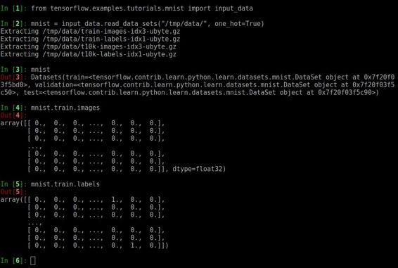
from tensorflow.examples.tutorials.mnist import input_data mnist = input_data.read_data_sets("/tmp/data/", one_hot=True) # Parameters learning_rate = 0.001 training_iters = 2000 batch_size = 128 display_step = 10 # Network Parameters n_input = 784 # MNIST data input (img shape: 28*28) n_classes = 10 # MNIST total classes (0-9 digits) 
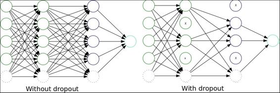
dropout = 0.75 # Dropout, probability to keep units # tf Graph input x = tf.placeholder(tf.float32, [None, n_input]) y = tf.placeholder(tf.float32, [None, n_classes]) keep_prob = tf.placeholder(tf.float32) #dropout (keep probability) #plt.imshow(X_train[1202].reshape((20, 20), order='F'), cmap='Greys', interpolation='nearest') # Create some wrappers for simplicity def conv2d(x, W, b, strides=1): # Conv2D wrapper, with bias and relu activation x = tf.nn.conv2d(x, W, strides=[1, strides, strides, 1], padding='SAME') x = tf.nn.bias_add(x, b) return tf.nn.relu(x) def maxpool2d(x, k=2): # MaxPool2D wrapper return tf.nn.max_pool(x, ksize=[1, k, k, 1], strides=[1, k, k, 1], padding='SAME') # Create model def conv_net(x, weights, biases, dropout): # Reshape input picture x = tf.reshape(x, shape=[-1, 28, 28, 1]) # Convolution Layer conv1 = conv2d(x, weights['wc1'], biases['bc1']) # Max Pooling (down-sampling) conv1 = maxpool2d(conv1, k=2) # Convolution Layer conv2 = conv2d(conv1, weights['wc2'], biases['bc2']) # Max Pooling (down-sampling) conv2 = maxpool2d(conv2, k=2) # Fully connected layer # Reshape conv2 output to fit fully connected layer input fc1 = tf.reshape(conv2, [-1, weights['wd1'].get_shape().as_list()[0]]) fc1 = tf.add(tf.matmul(fc1, weights['wd1']), biases['bd1']) fc1 = tf.nn.relu(fc1) # Apply Dropout fc1 = tf.nn.dropout(fc1, dropout) # Output, class prediction out = tf.add(tf.matmul(fc1, weights['out']), biases['out']) return out # Store layers weight & bias weights = { # 5x5 conv, 1 input, 32 outputs 'wc1': tf.Variable(tf.random_normal([5, 5, 1, 32])), # 5x5 conv, 32 inputs, 64 outputs 'wc2': tf.Variable(tf.random_normal([5, 5, 32, 64])), # fully connected, 7*7*64 inputs, 1024 outputs 'wd1': tf.Variable(tf.random_normal([7*7*64, 1024])), # 1024 inputs, 10 outputs (class prediction) 'out': tf.Variable(tf.random_normal([1024, n_classes])) } biases = { 'bc1': tf.Variable(tf.random_normal([32])), 'bc2': tf.Variable(tf.random_normal([64])), 'bd1': tf.Variable(tf.random_normal([1024])), 'out': tf.Variable(tf.random_normal([n_classes])) } # Construct model pred = conv_net(x, weights, biases, keep_prob) # Define loss and optimizer cost = tf.reduce_mean(tf.nn.softmax_cross_entropy_with_logits(pred, y)) optimizer = tf.train.AdamOptimizer(learning_rate=learning_rate).minimize(cost) # Evaluate model correct_pred = tf.equal(tf.argmax(pred, 1), tf.argmax(y, 1)) accuracy = tf.reduce_mean(tf.cast(correct_pred, tf.float32)) # Initializing the variables init = tf.initialize_all_variables() # Launch the graph with tf.Session() as sess: sess.run(init) step = 1 # Keep training until reach max iterations while step * batch_size < training_iters: batch_x, batch_y = mnist.train.next_batch(batch_size) test = batch_x[0] fig = plt.figure() plt.imshow(test.reshape((28, 28), order='C'), cmap='Greys', interpolation='nearest') print (weights['wc1'].eval()[0]) plt.imshow(weights['wc1'].eval()[0][0].reshape(4, 8), cmap='Greys', interpolation='nearest') # Run optimization op (backprop) sess.run(optimizer, feed_dict={x: batch_x, y: batch_y, keep_prob: dropout}) if step % display_step == 0: # Calculate batch loss and accuracy loss, acc = sess.run([cost, accuracy], feed_dict={x: batch_x, y: batch_y, keep_prob: 1.}) print "Iter " + str(step*batch_size) + ", Minibatch Loss= " + \ "{:.6f}".format(loss) + ", Training Accuracy= " + \ "{:.5f}".format(acc) step += 1 print "Optimization Finished!" # Calculate accuracy for 256 mnist test images print "Testing Accuracy:", \ sess.run(accuracy, feed_dict={x: mnist.test.images[:256], y: mnist.test.labels[:256], keep_prob: 1.})
In this example, we will be working on one of the most extensively used datasets in image comprehension, one which is used as a simple but general benchmark. In this example, we will build a simple CNN model to have an idea of the general structure of computations needed to tackle this type of classification problem.
This dataset consists of 40,000 images of 32x32 pixels, representing the following categories: airplane, automobile, bird, cat, deer, dog, frog, horse, ship, and truck. In this example, we will just take the first of the 10,000 image bundles to work on.
Here are some examples of the images you can find in the dataset:
We must make some data-structure adjustments to the original dataset, first by transforming it into a [10000, 3, 32, 32]
multidimensional array and then moving the channel dimension to the last order.
datadir='data/cifar-10-batches-bin/'
plt.ion()
G = glob.glob (datadir + '*.bin')
A = np.fromfile(G[0],dtype=np.uint8).reshape([10000,3073])
labels = A [:,0]
images = A [:,1:].reshape([10000,3,32,32]).transpose (0,2,3,1)
plt.imshow(images[14])
print labels[11]
images_unroll = A [:,1:]
Here, we will define our modeling function, which is a succession of convolution and pooling operations, with a final flattened layer and a logistic regression applied in order to determine the class probability of the current sample.
def conv_model (X, y): X= tf. reshape(X, [-1, 32, 32, 3]) with tf.variable_scope('conv_layer1'): h_conv1=tf.contrib.layers.conv2d(X, num_outputs=16, kernel_size=[5,5], activation_fn=tf.nn.relu)#print (h_conv1) h_pool1=max_pool_2x2(h_conv1)#print (h_pool1) with tf.variable_scope('conv_layer2'): h_conv2=tf.contrib.layers.conv2d(h_pool1, num_outputs=16, kernel_size=[5,5], activation_fn=tf.nn.relu) #print (h_conv2) h_pool2=max_pool_2x2(h_conv2) h_pool2_flat = tf.reshape(h_pool2, [-1,8*8*16 ]) h_fc1 = tf.contrib.layers.stack(h_pool2_flat, tf.contrib.layers.fully_connected ,[96,48], activation_fn=tf.nn.relu ) return skflow.models.logistic_regression(h_fc1,y)
The following is the function:
classifier = skflow.TensorFlowEstimator(model_fn=conv_model, n_classes=10, batch_size=100, steps=2000, learning_rate=0.01)
The following is the result:
Parameter |
Result 1 |
Result 2 |
CPU times |
user 35min 6s |
user 39.8 s |
sys |
1min 50s |
7.19 s |
total |
36min 57s |
47 s |
Wall time |
25min 3s |
32.5 s |
Accuracy |
0.612200
|
The following is the complete source code:
import glob import numpy as np import matplotlib.pyplot as plt import tensorflow as tf import tensorflow.contrib.learn as skflow from sklearn import metrics from tensorflow.contrib import learn datadir='data/cifar-10-batches-bin/' plt.ion() G = glob.glob (datadir + '*.bin') A = np.fromfile(G[0],dtype=np.uint8).reshape([10000,3073]) labels = A [:,0] images = A [:,1:].reshape([10000,3,32,32]).transpose (0,2,3,1) plt.imshow(images[15]) print labels[11] images_unroll = A [:,1:] def max_pool_2x2(tensor_in): return tf.nn.max_pool(tensor_in, ksize= [1,2,2,1], strides= [1,2,2,1], padding='SAME') def conv_model (X, y): X= tf. reshape(X, [-1, 32, 32, 3]) with tf.variable_scope('conv_layer1'): h_conv1=tf.contrib.layers.conv2d(X, num_outputs=16, kernel_size=[5,5], activation_fn=tf.nn.relu)#print (h_conv1) h_pool1=max_pool_2x2(h_conv1)#print (h_pool1) with tf.variable_scope('conv_layer2'): h_conv2=tf.contrib.layers.conv2d(h_pool1, num_outputs=16, kernel_size=[5,5], activation_fn=tf.nn.relu) #print (h_conv2) h_pool2=max_pool_2x2(h_conv2) h_pool2_flat = tf.reshape(h_pool2, [-1,8*8*16 ]) h_fc1 = tf.contrib.layers.stack(h_pool2_flat, tf.contrib.layers.fully_connected ,[96,48], activation_fn=tf.nn.relu ) return skflow.models.logistic_regression(h_fc1,y) images = np.array(images,dtype=np.float32) classifier = skflow.TensorFlowEstimator(model_fn=conv_model, n_classes=10, batch_size=100, steps=2000, learning_rate=0.01) %time classifier.fit(images, labels, logdir='/tmp/cnn_train/') %time score =metrics.accuracy_score(labels, classifier.predict(images))
In this chapter, we learned about one of the building blocks of the most advanced neural network architectures: convolutional neural networks. With this new tool, we worked on more complex datasets and concept abstractions, and so we will be able to understand state-of-the-art-models.
In the next chapter, we will be working with another new form of neural network and a part of a more recent neural network architecture: recurrent neural networks.