This is an area which is experiencing a blast on news techniques, and every day we hear of successful experiments applying DNN in solving new problems, for example, in computer vision, autonomous car driving, speech and text understanding, and so on.

In the previous chapters, we were using techniques that can be related with DNN, especially in the one covering Convolutional Neural Network.

For practical reasons, we will be referring to Deep Learning and Deep Neural Networks, to the architectures where the number of layers is significantly superior to a couple of similar layer, we will be referring to the Neural Network architectures with like tens of layer, or combinations of complex constructs.

The field of neural networks had been quite silent during the 1980s and the 1990s. There were some efforts, but the architectures were quite simple, and a big (and often not available) machine power was needed to try more complex approaches.

Around 1998, in Bells Labs, during research around the classification of hand written check digits, Ian LeCun started a new trend implementing the bases of what is considered Deep Learning - The Convolutional Neural Networks, which we have already studied in Chapter 5, Simple FeedForward Neural Networks .

In those years, SVM and other much more rigorously defined techniques were used to tackle those kinds of problems, but the fundamental paper on CNN, shows that Neural Networks could have a comparable or better performance compared to the then state of the art methods.

Alexnet can be seen as an augmented LeNet5, in the sense that its first layers with convolution operations. but add the not so used max pooling layers, and then a series of dense connected layers, building a last output class probability layer. The Visual Geometry Group (VGG) model

One of the other main contenders of the image classification challenge was the VGGof the University of Oxford.

The main characteristic of the VGG network architecture is that they reduced the size of the convolutional filters, to a simple 3x3, and combined them in sequences.

This idea of tiny convolutional kernels was disruptive to the initial ideas of the LeNet and its successor Alexnet, which used filters of up to 11x11 filters, much more complex and low in performance. This change in filter size was the beginning of a trend that is still current:

Summary of the parameter number per layer in VGG

However, this positive change of using a series of small convolution weights, the total setup amounted to a really big number of parameters (in the order of many millions) and so it had to be limited by a number of measures.

After two main research cycles dominated by Alexnet and VGG, Google disrupted the challenges with a very powerful architecture, Inception, which has several iterations.

The first of these iterations, started with its own version of Convolutional Neural Network layer-based architecture, called GoogLeNet, an architecture with a name reminiscent to the network approach that started it all.

1Inception module

GoogLeNet was the first iteration of this effort, and as you will see in the following figure, it has a very deep architecture, but it has the chilling sum of nine chained inception modules, with little or no modification:

Inception original architecture

Even being so complex, it managed to reduce the needed parameter number, and increased the accuracy, compared to Alexnet, which had been released just two years before.

The comprehension and scalability of this complex architecture is improved nevertheless, by the fact that almost all the structure consists of a determined arrangement and repetition of the same original structural layer building blocks.

The state of the art neural networks of 2015, while improving iteration over iteration, were having a problem of training instability.

In order to understand how the problems consisted, first we will remember the simple normalization steps that we applied in the previous examples. It basically consisted of centering the values on zero, and dividing by the maximum value, or the standard deviation, in order to have a good baseline for the gradients of the back propagations.

What occurs during the training of really large datasets, is that after a number of training examples, the different value oscillations begin to amplify the mean parameter value, like in a resonance phenomenon. What we very simply described is called a co variance shift.

Performance comparison with and without Batch Normalization

This is the main reason why the Batch Normalization techniques had been developed.

Again simplifying the process description, it consists of applying normalizations not only to the original input values, it also normalizes the output values at each layer, avoiding the instabilities appearing between layers, before they begin to affect or drift the values.

This is the main feature that Google shipped in its improved implementation of GoogLeNet, released in February 2015, and it is also called Inception V2.

• Reduce the number of convolutions to maximum 3x3
• Increase the general depth of the networks
• Use the width increase technique at each layer to improve feature combination

There are a big number of recently developed neural network architectures; in fact, the field is so dynamic that we have more or less a new outstanding architecture apparition every year. A list of the most promising neural network architectures are:

scipy.io.loadmat(file_name, mdict=None, appendmat=True, **kwargs) 

For the solution of this problem, we will be using a pre-trained dataset, that is, the retrained coefficients of a VGG neural network, with the Imagenet dataset.

Given that the coefficients are given in the loaded parameter matrix, there is not much work to do regarding the initial dataset.

The modeling architecture is divided mainly in two parts: the style and the content.

For the generation of the final images, a VGG network without the final fully connected layer is used.

This architecture defines two different loss functions to optimize the two different aspects of the final image, one for the content and one for the style.

 # content loss 
        content_loss = content_weight * (2 * tf.nn.l2_loss( 
                net[CONTENT_LAYER] - content_features[CONTENT_LAYER]) / 
                content_features[CONTENT_LAYER].size) 
 

In this example, we will just check for the number of indicated iterations (the iterations parameter).

For the execution of this program for a good (around 1000) iteration number, we recommend to have at least 8GB of RAM memory available:

python neural_style.py --content examples/2-content.jpg --styles examples/2-style1.jpg  --checkpoint-iterations=100 --iterations=1000 --checkpoint-output=out%s.jpg --output=outfinal

The results for the preceding command is as follows:

Style transfer steps

The console output is as follows:

Iteration 1/1000
Iteration 2/1000
Iteration 3/1000
Iteration 4/1000
...
Iteration 999/1000
Iteration 1000/1000
  content loss: 908786
    style loss: 261789
       tv loss: 25639.9
    total loss: 1.19621e+06

The code for neural_style.py is as follows:

import os 
 
import numpy as np 
import scipy.misc 
 
from stylize import stylize 
 
import math 
from argparse import ArgumentParser 
 
# default arguments 
CONTENT_WEIGHT = 5e0 
STYLE_WEIGHT = 1e2 
TV_WEIGHT = 1e2 
LEARNING_RATE = 1e1 
STYLE_SCALE = 1.0 
ITERATIONS = 100 
VGG_PATH = 'imagenet-vgg-verydeep-19.mat' 
 
 
def build_parser(): 
    parser = ArgumentParser() 
    parser.add_argument('--content', 
            dest='content', help='content image', 
            metavar='CONTENT', required=True) 
    parser.add_argument('--styles', 
            dest='styles', 
            nargs='+', help='one or more style images', 
            metavar='STYLE', required=True) 
    parser.add_argument('--output', 
            dest='output', help='output path', 
            metavar='OUTPUT', required=True) 
    parser.add_argument('--checkpoint-output', 
            dest='checkpoint_output', help='checkpoint output format', 
            metavar='OUTPUT') 
    parser.add_argument('--iterations', type=int, 
            dest='iterations', help='iterations (default %(default)s)', 
            metavar='ITERATIONS', default=ITERATIONS) 
    parser.add_argument('--width', type=int, 
            dest='width', help='output width', 
            metavar='WIDTH') 
    parser.add_argument('--style-scales', type=float, 
            dest='style_scales', 
            nargs='+', help='one or more style scales', 
            metavar='STYLE_SCALE') 
    parser.add_argument('--network', 
            dest='network', help='path to network parameters (default %(default)s)', 
            metavar='VGG_PATH', default=VGG_PATH) 
    parser.add_argument('--content-weight', type=float, 
            dest='content_weight', help='content weight (default %(default)s)', 
            metavar='CONTENT_WEIGHT', default=CONTENT_WEIGHT) 
    parser.add_argument('--style-weight', type=float, 
            dest='style_weight', help='style weight (default %(default)s)', 
            metavar='STYLE_WEIGHT', default=STYLE_WEIGHT) 
    parser.add_argument('--style-blend-weights', type=float, 
            dest='style_blend_weights', help='style blending weights', 
            nargs='+', metavar='STYLE_BLEND_WEIGHT') 
    parser.add_argument('--tv-weight', type=float, 
            dest='tv_weight', help='total variation regularization weight (default %(default)s)', 
            metavar='TV_WEIGHT', default=TV_WEIGHT) 
    parser.add_argument('--learning-rate', type=float, 
            dest='learning_rate', help='learning rate (default %(default)s)', 
            metavar='LEARNING_RATE', default=LEARNING_RATE) 
    parser.add_argument('--initial', 
            dest='initial', help='initial image', 
            metavar='INITIAL') 
    parser.add_argument('--print-iterations', type=int, 
            dest='print_iterations', help='statistics printing frequency', 
            metavar='PRINT_ITERATIONS') 
    parser.add_argument('--checkpoint-iterations', type=int, 
            dest='checkpoint_iterations', help='checkpoint frequency', 
            metavar='CHECKPOINT_ITERATIONS') 
    return parser 
 
 
def main(): 
    parser = build_parser() 
    options = parser.parse_args() 
 
    if not os.path.isfile(options.network): 
        parser.error("Network %s does not exist. (Did you forget to download it?)" % options.network) 
 
    content_image = imread(options.content) 
    style_images = [imread(style) for style in options.styles] 
 
    width = options.width 
    if width is not None: 
        new_shape = (int(math.floor(float(content_image.shape[0]) / 
                content_image.shape[1] * width)), width) 
        content_image = scipy.misc.imresize(content_image, new_shape) 
    target_shape = content_image.shape 
    for i in range(len(style_images)): 
        style_scale = STYLE_SCALE 
        if options.style_scales is not None: 
            style_scale = options.style_scales[i] 
        style_images[i] = scipy.misc.imresize(style_images[i], style_scale * 
                target_shape[1] / style_images[i].shape[1]) 
 
    style_blend_weights = options.style_blend_weights 
    if style_blend_weights is None: 
        # default is equal weights 
        style_blend_weights = [1.0/len(style_images) for _ in style_images] 
    else: 
        total_blend_weight = sum(style_blend_weights) 
        style_blend_weights = [weight/total_blend_weight 
                               for weight in style_blend_weights] 
 
    initial = options.initial 
    if initial is not None: 
        initial = scipy.misc.imresize(imread(initial), content_image.shape[:2]) 
 
    if options.checkpoint_output and "%s" not in options.checkpoint_output: 
        parser.error("To save intermediate images, the checkpoint output " 
                     "parameter must contain `%s` (e.g. `foo%s.jpg`)") 
 
    for iteration, image in stylize( 
        network=options.network, 
        initial=initial, 
        content=content_image, 
        styles=style_images, 
        iterations=options.iterations, 
        content_weight=options.content_weight, 
        style_weight=options.style_weight, 
        style_blend_weights=style_blend_weights, 
        tv_weight=options.tv_weight, 
        learning_rate=options.learning_rate, 
        print_iterations=options.print_iterations, 
        checkpoint_iterations=options.checkpoint_iterations 
    ): 
        output_file = None 
        if iteration is not None: 
            if options.checkpoint_output: 
                output_file = options.checkpoint_output % iteration 
        else: 
            output_file = options.output 
        if output_file: 
            imsave(output_file, image) 
 
 
def imread(path): 
    return scipy.misc.imread(path).astype(np.float) 
 
 
def imsave(path, img): 
    img = np.clip(img, 0, 255).astype(np.uint8) 
    scipy.misc.imsave(path, img) 
 
 
if __name__ == '__main__': 
    main() 

The code for Stilize.py is as follows:

import vgg 
 
import tensorflow as tf 
import numpy as np 
 
from sys import stderr 
 
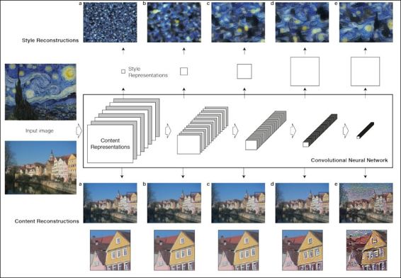
CONTENT_LAYER = 'relu4_2' 
STYLE_LAYERS = ('relu1_1', 'relu2_1', 'relu3_1', 'relu4_1', 'relu5_1') 
 
 
try: 
    reduce 
except NameError: 
    from functools import reduce 
 
 
def stylize(network, initial, content, styles, iterations, 
        content_weight, style_weight, style_blend_weights, tv_weight, 
        learning_rate, print_iterations=None, checkpoint_iterations=None): 
    """ 
    Stylize images. 
 
    This function yields tuples (iteration, image); `iteration` is None 
    if this is the final image (the last iteration).  Other tuples are yielded 
    every `checkpoint_iterations` iterations. 
 
    :rtype: iterator[tuple[int|None,image]] 
    """ 
    shape = (1,) + content.shape 
    style_shapes = [(1,) + style.shape for style in styles] 
    content_features = {} 
    style_features = [{} for _ in styles] 
 
    # compute content features in feedforward mode 
    g = tf.Graph() 
    with g.as_default(), g.device('/cpu:0'), tf.Session() as sess: 
        image = tf.placeholder('float', shape=shape) 
        net, mean_pixel = vgg.net(network, image) 
        content_pre = np.array([vgg.preprocess(content, mean_pixel)]) 
        content_features[CONTENT_LAYER] = net[CONTENT_LAYER].eval( 
                feed_dict={image: content_pre}) 
 
    # compute style features in feedforward mode 
    for i in range(len(styles)): 
        g = tf.Graph() 
        with g.as_default(), g.device('/cpu:0'), tf.Session() as sess: 
            image = tf.placeholder('float', shape=style_shapes[i]) 
            net, _ = vgg.net(network, image) 
            style_pre = np.array([vgg.preprocess(styles[i], mean_pixel)]) 
            for layer in STYLE_LAYERS: 
                features = net[layer].eval(feed_dict={image: style_pre}) 
                features = np.reshape(features, (-1, features.shape[3])) 
                gram = np.matmul(features.T, features) / features.size 
                style_features[i][layer] = gram 
 
    # make stylized image using backpropogation 
    with tf.Graph().as_default(): 
        if initial is None: 
            noise = np.random.normal(size=shape, scale=np.std(content) * 0.1) 
            initial = tf.random_normal(shape) * 0.256 
        else: 
            initial = np.array([vgg.preprocess(initial, mean_pixel)]) 
            initial = initial.astype('float32') 
        image = tf.Variable(initial) 
        net, _ = vgg.net(network, image) 
 
        # content loss 
        content_loss = content_weight * (2 * tf.nn.l2_loss( 
                net[CONTENT_LAYER] - content_features[CONTENT_LAYER]) / 
                content_features[CONTENT_LAYER].size) 
        # style loss 
        style_loss = 0 
        for i in range(len(styles)): 
            style_losses = [] 
            for style_layer in STYLE_LAYERS: 
                layer = net[style_layer] 
                _, height, width, number = map(lambda i: i.value, layer.get_shape()) 
                size = height * width * number 
                feats = tf.reshape(layer, (-1, number)) 
                gram = tf.matmul(tf.transpose(feats), feats) / size 
                style_gram = style_features[i][style_layer] 
                style_losses.append(2 * tf.nn.l2_loss(gram - style_gram) / style_gram.size) 
            style_loss += style_weight * style_blend_weights[i] * reduce(tf.add, style_losses) 
        # total variation denoising 
        tv_y_size = _tensor_size(image[:,1:,:,:]) 
        tv_x_size = _tensor_size(image[:,:,1:,:]) 
        tv_loss = tv_weight * 2 * ( 
                (tf.nn.l2_loss(image[:,1:,:,:] - image[:,:shape[1]-1,:,:]) / 
                    tv_y_size) + 
                (tf.nn.l2_loss(image[:,:,1:,:] - image[:,:,:shape[2]-1,:]) / 
                    tv_x_size)) 
        # overall loss 
        loss = content_loss + style_loss + tv_loss 
 
        # optimizer setup 
        train_step = tf.train.AdamOptimizer(learning_rate).minimize(loss) 
 
        def print_progress(i, last=False): 
            stderr.write('Iteration %d/%d\n' % (i + 1, iterations)) 
            if last or (print_iterations and i % print_iterations == 0): 
                stderr.write('  content loss: %g\n' % content_loss.eval()) 
                stderr.write('    style loss: %g\n' % style_loss.eval()) 
                stderr.write('       tv loss: %g\n' % tv_loss.eval()) 
                stderr.write('    total loss: %g\n' % loss.eval()) 
 
        # optimization 
        best_loss = float('inf') 
        best = None 
        with tf.Session() as sess: 
            sess.run(tf.initialize_all_variables()) 
            for i in range(iterations): 
                last_step = (i == iterations - 1) 
                print_progress(i, last=last_step) 
                train_step.run() 
 
                if (checkpoint_iterations and i % checkpoint_iterations == 0) or last_step: 
                    this_loss = loss.eval() 
                    if this_loss < best_loss: 
                        best_loss = this_loss 
                        best = image.eval() 
                    yield ( 
                        (None if last_step else i), 
                        vgg.unprocess(best.reshape(shape[1:]), mean_pixel) 
                    ) 
 
 
def _tensor_size(tensor): 
    from operator import mul 
    return reduce(mul, (d.value for d in tensor.get_shape()), 1) 
 vgg.py 
import tensorflow as tf 
import numpy as np 
import scipy.io 
 
 
def net(data_path, input_image): 
    layers = ( 
        'conv1_1', 'relu1_1', 'conv1_2', 'relu1_2', 'pool1', 
 
        'conv2_1', 'relu2_1', 'conv2_2', 'relu2_2', 'pool2', 
 
        'conv3_1', 'relu3_1', 'conv3_2', 'relu3_2', 'conv3_3', 
        'relu3_3', 'conv3_4', 'relu3_4', 'pool3', 
 
        'conv4_1', 'relu4_1', 'conv4_2', 'relu4_2', 'conv4_3', 
        'relu4_3', 'conv4_4', 'relu4_4', 'pool4', 
 
        'conv5_1', 'relu5_1', 'conv5_2', 'relu5_2', 'conv5_3', 
        'relu5_3', 'conv5_4', 'relu5_4' 
    ) 
 
    data = scipy.io.loadmat(data_path) 
    mean = data['normalization'][0][0][0] 
    mean_pixel = np.mean(mean, axis=(0, 1)) 
    weights = data['layers'][0] 
 
    net = {} 
    current = input_image 
    for i, name in enumerate(layers): 
        kind = name[:4] 
        if kind == 'conv': 
            kernels, bias = weights[i][0][0][0][0] 
            # matconvnet: weights are [width, height, in_channels, out_channels] 
            # tensorflow: weights are [height, width, in_channels, out_channels] 
            kernels = np.transpose(kernels, (1, 0, 2, 3)) 
            bias = bias.reshape(-1) 
            current = _conv_layer(current, kernels, bias) 
        elif kind == 'relu': 
            current = tf.nn.relu(current) 
        elif kind == 'pool': 
            current = _pool_layer(current) 
        net[name] = current 
 
    assert len(net) == len(layers) 
    return net, mean_pixel 
 
def _conv_layer(input, weights, bias): 
    conv = tf.nn.conv2d(input, tf.constant(weights), strides=(1, 1, 1, 1), 
            padding='SAME') 
    return tf.nn.bias_add(conv, bias) 
 
def _pool_layer(input): 
    return tf.nn.max_pool(input, ksize=(1, 2, 2, 1), strides=(1, 2, 2, 1), 
            padding='SAME') 
 
 
def preprocess(image, mean_pixel): 
    return image - mean_pixel 
 
 
def unprocess(image, mean_pixel): 
    return image + mean_pixel