Until now, we have been running code that runs on the host computer's main CPU. This implies that, at most, we use all the different processor cores (2 or 4 for low-end processors, up to 16 in more advanced processors).
In the last decade, the General Processing Unit, or GPU, has become a ubiquitous part of any high performance computing setup. Its massive, intrinsic parallelism is very well suited for the high dimension matrix multiplications and other operations required in machine learning model training and running.
Nevertheless, even having really powerful computing nodes there is a large number of tasks with which even the most powerful individual server can't cope.
For this reason, a distributed way of training and running a model had to be developed. This is the original function of distributed TensorFlow.
In this chapter, you will:
Before trying to perform calculations, TensorFlow allows you to log all the available resources. In this way we can apply operations only in existing computing types.
In order to obtain a log of the computing elements on a machine, we can use the log_device_placement flag when we create a TensorFlow session, in this way:
python
>>>Import tensorflow as tf
>>>sess = tf.Session(config=tf.ConfigProto(log_device_placement=True))
This is the output of the commands:
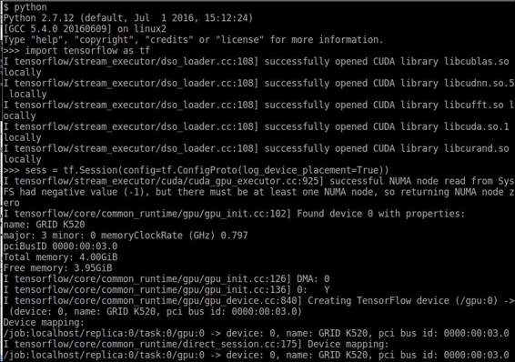
Selecting a GPU to run code
This long output mainly shows the loading of the different needed CUDA library, and then the name (GRID K520) and the computing capabilities of the GPU.
If we have a GPU available, but still want to continue working with the CPU, we can select one via the method, tf.Graph.device.
The method call is the following:
tf.Graph.device(device_name_or_function) :
This function receives a processing unit string, a function returning a processing unit string, or none, and returns a context manager with the processing unit assigned.
If the parameter is a function, each operation will call this function to decide in which processing unit it will execute, a useful element to combine all operations.
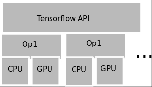
To specify which computing unit we are referring to when specifying a device, TensorFlow uses a simple scheme with the following format:
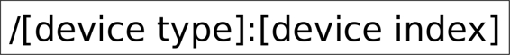
Device ID format
Example device identification includes:
When available, if nothing is indicated to the contrary, the first GPU device is used.
In this example, we will create two tensors, locate the existing GPU as the default location, and will execute the tensor sum on it on a server configured with the CUDA environment (which you will learn to install in Appendix A - Library Installation and Additional Tips).
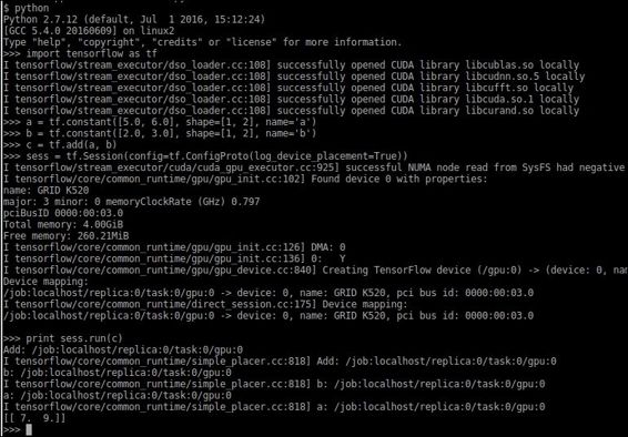
Here we see that both the constants and the sum operation are built on the /gpu:0 server. This is because the GPU is the preferred computing device type when available.
This example will serve as an introduction of parallel processing, implementing the Monte Carlo approximation of Pi.
Monte Carlo utilizes a random number sequence to perform an approximation.
In order to solve this problem, we will throw many random samples, knowing that the ratio of samples inside the circle over the ones on the square, is the same as the area ratio.
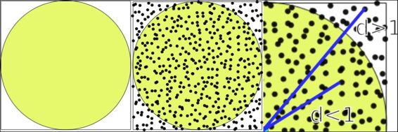
Random area calculation techniques
The calculation assumes that if the probability distribution is uniform, the number of samples assigned is proportional to the area of the figures.
We use the following proportion:

Area proportion for Pi calculation
From the aforementioned proportion, we infer that number of sample in the circle/number of sample of square is also 0.78.
An additional fact is that the more random samples we can generate for the calculation, the more approximate the answer. This is when incrementing the number of GPUs will give us more samples and accuracy.
A further reduction that we do is that we generate (X,Y) coordinates, ranging from (0..1), so the random number generation is more direct. So the only criteria we need to determine if a sample belongs to the circle is distance = d < 1.0 (radius of the circle).
This solution will be based around the CPU; it will manage the GPU resources that we have in the server (in this case, 4) and then we will receive the results, doing the final sample sum.
Note: This method has a really slow convergence rate of O(n1/2), but will be used as an example, given its simplicity.
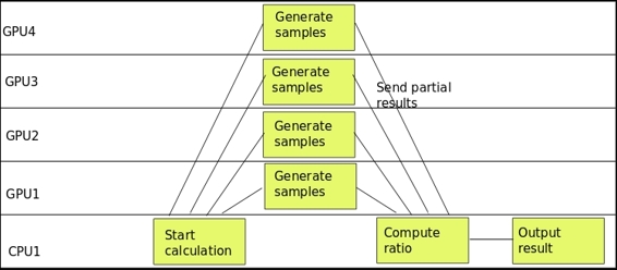
Computing tasks timeline
In the preceding figure, we see the parallel behavior of the calculation, being the sample generation and counting the main activity.
The source code is as follows:
import tensorflow as tf
import numpy as np
c = []
#Distribute the work between the GPUs
for d in ['/gpu:0', '/gpu:1', '/gpu:2', '/gpu:3']:
    #Generate the random 2D samples
    i=tf.constant(np.random.uniform(size=10000), shape=[5000,2])
    with tf.Session() as sess:
        tf.initialize_all_variables()
        #Calculate the euclidean distance to the origin
        distances=tf.reduce_sum(tf.pow(i,2),1)
        #Sum the samples inside the circle
        tempsum = sess.run(tf.reduce_sum(tf.cast(tf.greater_equal(tf.cast(1.0,tf.float64),distances),tf.float64)))
        #append the current result to the results array
        c.append( tempsum)
    #Do the final ratio calculation on the CPU
    with tf.device('/cpu:0'):
        with tf.Session() as sess:
            sum = tf.add_n(c)
            print (sess.run(sum/20000.0)*4.0)
Distributed TensorFlow is a complementary technology, which aims to easily and efficiently create clusters of computing nodes, and to distribute the jobs between nodes in a seamless way.
It is the standard way to create distributed computing environments, and to execute the training and running of models at a massive scale, so it's very important to be able to do the main task found in production, high volume data setups.
In this section, we will describe all the components on a distributed TensorFlow computing setup, from the most fine-grained task elements, to the whole cluster description.
Jobs define a group of homogeneous tasks, normally aimed to the same subset of the problem-solving area.
Examples of job distinctions are:
Tasks are subdivisions of jobs, which perform the different steps or parallel work units to solve the problem area of its job, and are normally attached to a single process.
Every job has a number of tasks, and they are identified by an index. Normally the task with the index 0, is considered the main or coordinator task.
Server are logical objects representing a set of physical devices dedicated to implementing tasks. A server will be exclusively assigned to a single task.
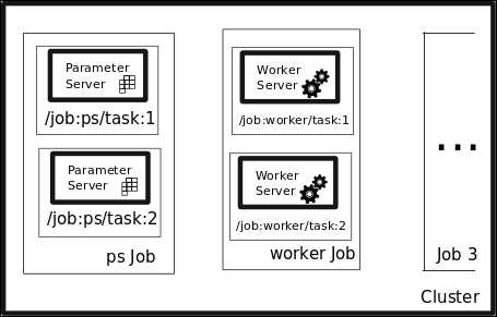
In the following figure, we will represent all the participating parts in a cluster computing setup:
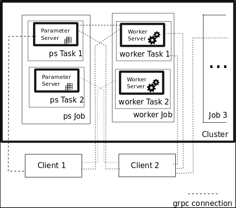
TensorFlow cluster setup elements
The figure contains the two jobs represented by the ps and the worker jobs, and the grpc communication channels (covered in Appendix A - Library Installation and Additional Tips) that can be created from the clients for them. For every job type, there are servers implementing different tasks, which solve subsets of the job's domain problem.
The first task for a distributed cluster program will be defining and creating a ClusterSpec object, which contains the real server instance's addresses and ports, which will be a part of the cluster.
The two main ways of defining this ClusterSpec are:
tf.train.ClusterSpec object, which specifies all cluster taskstf.train.Server, and relating the local task with a job name plus task indexClusterSpec objects are defined using the protocol buffer format, which is a special format based on JSON.
The format is the following:
{
    "job1 name": [
        "task0 server uri",
        "task1 server uri"
         ...
    ]
...
    "jobn name"[
        "task0 server uri",
        "task1 server uri"
    ]})
...
So this would be the function call to create a cluster with a parameter server task server and three worker task servers:
tf.train.ClusterSpec({
    "worker": [
        "wk0.example.com:2222",
        "wk1.example.com:2222",
        "wk2.example.com:2222"
    ],
    "ps": [
        "ps0.example.com:2222",
    ]})
After we create the ClusterSpec, we now have an exact idea of the cluster configuration, in the runtime. We will proceed to create the local server instance, creating an instance of tf.train.Server:
This is a sample server creation, which takes a cluster object, a job name, and a task index as a parameter:
server = tf.train.Server(cluster, job_name="local", task_index=[Number of server])
In order to begin learning the operation of the cluster, we need to learn the addressing of the computing resources.
First of all, we suppose we have already created a cluster, with its different resources of jobs and tasks. The ID string for any of the resources has the following form:
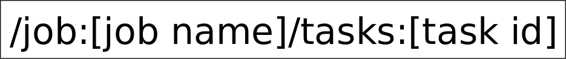
And the normal invocation of the resource in a context manager is the with keyword, with the following structure.
with tf.device("/job:ps/task:1"):
  [Code Block]
The with keyword indicates that whenever a task identifier is needed, the one specified in the context manager directive will be used.
The following figure illustrates a sample cluster setup, with the addressing names of all the different parts of the setup:
Server elements naming
This sample code will show you the approximate structure of a program addressing different tasks in a cluster, specifically a parameter server and a worker job:
#Address the Parameter Server task
with tf.device("/job:ps/task:1"):
  weights = tf.Variable(...)
  bias = tf.Variable(...)

#Address the Parameter Server task
with tf.device("/job:worker/task:1"):
    #... Generate and train a model
  layer_1 = tf.nn.relu(tf.matmul(input, weights_1) + biases_1)
  logits = tf.nn.relu(tf.matmul(layer_1, weights_2) + biases_2)
  train_op = ...

#Command the main task of the cluster
with tf.Session("grpc://worker1.cluster:2222") as sess:
  for i in range(100):
    sess.run(train_op)
In this example, we will change the perspective, going from one server with several computing resources, to a cluster of servers with a number of resources for each one.
The execution of the distributed version will have a different setup, explained in the following figure:
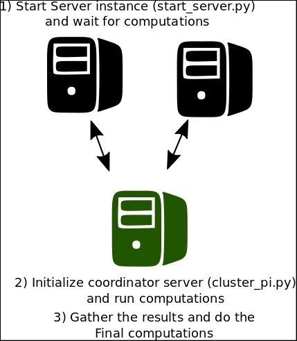
Distributed coordinated running
This script will be executed on each one of the computation nodes, which will generate a batch of samples, augmenting the number of generated random numbers by the number of available servers. In this case, we will use two servers and we suppose we initiate them in the localhost, indicating in the command-line the index number. If you want to run them in separate nodes, you just have to replace the localhost addresses in the ClusterSpec definition (and the name if you want it to be more representative).
The source code for the script is as follows:
import tensorflow as tf
tf.app.flags.DEFINE_string("index", "0","Server index")
FLAGS = tf.app.flags.FLAGS
print FLAGS.index
cluster = tf.train.ClusterSpec({"local": ["localhost:2222", "localhost:2223"]})
server = tf.train.Server(cluster, job_name="local", task_index=int(FLAGS.index))
server.join()
The command lines for executing this script in localhost are as follows:
python start_server.py -index=0 #Server  task 0
python start_server.py -index=1 #Server task 1
This is the expected output for one of the servers:
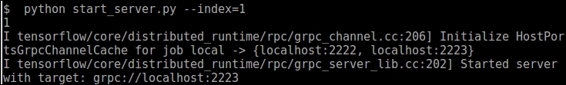
Individual server starting command line
The source code is as follows:
import tensorflow as tf
import numpy as np

tf.app.flags.DEFINE_integer("numsamples", "100","Number of samples per server")
FLAGS = tf.app.flags.FLAGS

print ("Sample number per server: " + str(FLAGS.numsamples)  )
cluster = tf.train.ClusterSpec({"local": ["localhost:2222", "localhost:2223"]})
#This is the list containing the sumation of samples on any node
c=[]

def generate_sum():
        i=tf.constant(np.random.uniform(size=FLAGS.numsamples*2), shape=[FLAGS.numsamples,2])
        distances=tf.reduce_sum(tf.pow(i,2),1)
        return (tf.reduce_sum(tf.cast(tf.greater_equal(tf.cast(1.0,tf.float64),distances),tf.int32)))


with tf.device("/job:local/task:0"):
        test1= generate_sum()

with tf.device("/job:local/task:1"):
        test2= generate_sum()
#If your cluster is local, you must replace localhost by the address of the first node
with tf.Session("grpc://localhost:2222") as sess:
      result = sess.run(tf.cast(test1 + test2,tf.float64)/FLAGS.numsamples*2.0)
      print(result)
This very simple example will serve us as an example of how the pieces of a distributed TensorFlow setup work.
In this sample, we will do a very simple task, which nevertheless takes all the needed steps in a machine learning process.
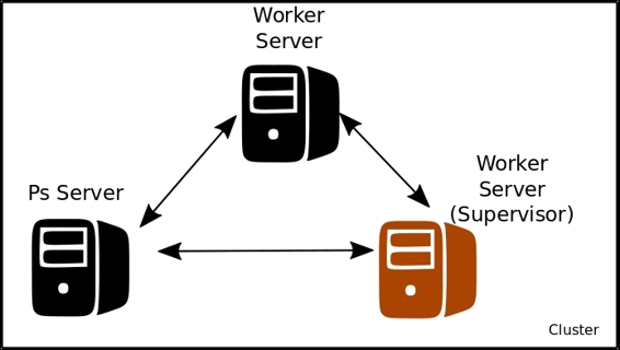
Distributed training cluster setup
The Ps Server will contain the different parameters of the linear function to solve (in this case just x and b0), and the two worker servers will do the training of the variable, which will constantly update and improve upon the last one, working on a collaboration mode.
The sample code is as follows:
import tensorflow as tf
import numpy as np
from sklearn.utils import shuffle

# Here we define our cluster setup via the command line
tf.app.flags.DEFINE_string("ps_hosts", "",
                           "Comma-separated list of hostname:port pairs")
tf.app.flags.DEFINE_string("worker_hosts", "",
                           "Comma-separated list of hostname:port pairs")

# Define the characteristics of the cluster node, and its task index
tf.app.flags.DEFINE_string("job_name", "", "One of 'ps', 'worker'")
tf.app.flags.DEFINE_integer("task_index", 0, "Index of task within the job")

FLAGS = tf.app.flags.FLAGS


def main(_):
  ps_hosts = FLAGS.ps_hosts.split(",")
  worker_hosts = FLAGS.worker_hosts.split(",")

  # Create a cluster following the command line paramaters.
  cluster = tf.train.ClusterSpec({"ps": ps_hosts, "worker": worker_hosts})

  # Create the local task.
  server = tf.train.Server(cluster,
                           job_name=FLAGS.job_name,
                           task_index=FLAGS.task_index)

  if FLAGS.job_name == "ps":
    server.join()
  elif FLAGS.job_name == "worker":

    # Assigns ops to the local worker by default.
    with tf.device(tf.train.replica_device_setter(
        worker_device="/job:worker/task:%d" % FLAGS.task_index,
        cluster=cluster)):

      #Define the training set, and the model parameters, loss function and training operation
      trX = np.linspace(-1, 1, 101)
      trY = 2 * trX + np.random.randn(*trX.shape) * 0.4 + 0.2 # create a y value
      X = tf.placeholder("float", name="X") # create symbolic variables
      Y = tf.placeholder("float", name = "Y")

      def model(X, w, b):
        return tf.mul(X, w) + b # We just define the line as X*w + b0

      w = tf.Variable(-1.0, name="b0") # create a shared variable
      b = tf.Variable(-2.0, name="b1") # create a shared variable
      y_model = model(X, w, b)

      loss = (tf.pow(Y-y_model, 2)) # use sqr error for cost function
      global_step = tf.Variable(0)

      train_op = tf.train.AdagradOptimizer(0.8).minimize(
          loss, global_step=global_step)

    #Create a saver, and a summary and init operation
      saver = tf.train.Saver()
      summary_op = tf.merge_all_summaries()
      init_op = tf.initialize_all_variables()

    # Create a "supervisor", which oversees the training process.
    sv = tf.train.Supervisor(is_chief=(FLAGS.task_index == 0),
                             logdir="/tmp/train_logs",
                             init_op=init_op,
                             summary_op=summary_op,
                             saver=saver,
                             global_step=global_step,
                             save_model_secs=600)

    # The supervisor takes care of session initialization, restoring from
    # a checkpoint, and closing when done or an error occurs.
    with sv.managed_session(server.target) as sess:
      # Loop until the supervisor shuts down
      step = 0
      while not sv.should_stop() :
        # Run a training step asynchronously.
        # See `tf.train.SyncReplicasOptimizer` for additional details on how to
        # perform *synchronous* training.
        for i in range(100):
          trX, trY = shuffle (trX, trY, random_state=0)
          for (x, y) in zip(trX, trY):
              _, step = sess.run([train_op, global_step],feed_dict={X: x, Y: y})
          #Print the partial results, and the current node doing the calculation
          print ("Partial result from node: " + str(FLAGS.task_index) + ", w: " + str(w.eval(session=sess))+ ", b0: " + str(b.eval(session=sess)))
    # Ask for all the services to stop.
    sv.stop()


if __name__ == "__main__":
  tf.app.run()
In the parameter server current host:
python trainer.py  --ps_hosts=localhost:2222   --worker_hosts=localhost:2223,localhost:2224   --job_name=ps -task_index=0
he first
In the worker host number one:
python trainer.py --ps_hosts=localhost:2222 --worker_hosts=localhost:2223,localhost:2224 --job_name=worker -task_index=0
In the worker host number two:
python trainer.py --ps_hosts=localhost:2222 --worker_hosts=localhost:2223,localhost:2224 --job_name=worker --task_index=1
In this chapter, we have reviewed the two main elements we have in the TensorFlow toolbox to implement our models in a high performance environment, be it in single servers or a distributed cluster environment.
In the following chapter, we will review detailed instructions about how to install TensorFlow under a variety of environments and tools.