numpy.linalg.lstsq
-
numpy.linalg.lstsq(a, b, rcond=-1)[source]¶ Return the least-squares solution to a linear matrix equation.
Solves the equation a x = b by computing a vector x that minimizes the Euclidean 2-norm || b - a x ||^2. The equation may be under-, well-, or over- determined (i.e., the number of linearly independent rows of a can be less than, equal to, or greater than its number of linearly independent columns). If a is square and of full rank, then x (but for round-off error) is the “exact” solution of the equation.
Parameters: a : (M, N) array_like
“Coefficient” matrix.
b : {(M,), (M, K)} array_like
Ordinate or “dependent variable” values. If b is two-dimensional, the least-squares solution is calculated for each of the K columns of b.
rcond : float, optional
Cut-off ratio for small singular values of a. Singular values are set to zero if they are smaller than rcond times the largest singular value of a.
Returns: x : {(N,), (N, K)} ndarray
Least-squares solution. If b is two-dimensional, the solutions are in the K columns of x.
residuals : {(), (1,), (K,)} ndarray
Sums of residuals; squared Euclidean 2-norm for each column in
b - a*x. If the rank of a is < N or M <= N, this is an empty array. If b is 1-dimensional, this is a (1,) shape array. Otherwise the shape is (K,).rank : int
Rank of matrix a.
s : (min(M, N),) ndarray
Singular values of a.
Raises: LinAlgError
If computation does not converge.
Notes
If b is a matrix, then all array results are returned as matrices.
Examples
Fit a line,
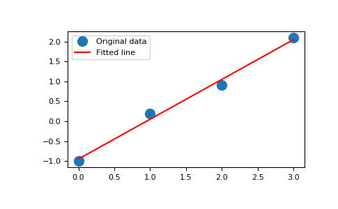
y = mx + c, through some noisy data-points:>>> x = np.array([0, 1, 2, 3]) >>> y = np.array([-1, 0.2, 0.9, 2.1])
By examining the coefficients, we see that the line should have a gradient of roughly 1 and cut the y-axis at, more or less, -1.
We can rewrite the line equation as
y = Ap, whereA = [[x 1]]andp = [[m], [c]]. Now uselstsqto solve for p:>>> A = np.vstack([x, np.ones(len(x))]).T >>> A array([[ 0., 1.], [ 1., 1.], [ 2., 1.], [ 3., 1.]])
>>> m, c = np.linalg.lstsq(A, y)[0]
>>> print(m, c)
1.0 -0.95
Plot the data along with the fitted line:
>>> import matplotlib.pyplot as plt
>>> plt.plot(x, y, 'o', label='Original data', markersize=10)
>>> plt.plot(x, m*x + c, 'r', label='Fitted line')
>>> plt.legend()
>>> plt.show()
(Source code, png, pdf)