numpy.random.RandomState.vonmises¶

RandomState.vonmises(mu, kappa, size=None)¶

Draw samples from a von Mises distribution.

Samples are drawn from a von Mises distribution with specified mode (mu) and dispersion (kappa), on the interval [-pi, pi].

The von Mises distribution (also known as the circular normal distribution) is a continuous probability distribution on the unit circle. It may be thought of as the circular analogue of the normal distribution.

Parameters:	mu : float Mode (“center”) of the distribution. kappa : float Dispersion of the distribution, has to be >=0. size : int or tuple of ints, optional Output shape. If the given shape is, e.g., `(m, n, k)`, then `m * n * k` samples are drawn. Default is None, in which case a single value is returned.
Returns:	samples : scalar or ndarray The returned samples, which are in the interval [-pi, pi].

Parameters:

mu : float

Mode (“center”) of the distribution.

kappa : float

Dispersion of the distribution, has to be >=0.

size : int or tuple of ints, optional

Output shape. If the given shape is, e.g., (m, n, k), then m * n * k samples are drawn. Default is None, in which case a single value is returned.

Returns:

samples : scalar or ndarray

The returned samples, which are in the interval [-pi, pi].

See also

scipy.stats.distributions.vonmises: probability density function, distribution, or cumulative density function, etc.

Notes

The probability density for the von Mises distribution is

where $\mu$ is the mode and $\kappa$ the dispersion, and $I_0(\kappa)$ is the modified Bessel function of order 0.

The von Mises is named for Richard Edler von Mises, who was born in Austria-Hungary, in what is now the Ukraine. He fled to the United States in 1939 and became a professor at Harvard. He worked in probability theory, aerodynamics, fluid mechanics, and philosophy of science.

References

[R199]

Abramowitz, M. and Stegun, I. A. (Eds.). “Handbook of Mathematical Functions with Formulas, Graphs, and Mathematical Tables, 9th printing,” New York: Dover, 1972.

[R200]

von Mises, R., “Mathematical Theory of Probability and Statistics”, New York: Academic Press, 1964.

Examples

Draw samples from the distribution:

>>> mu, kappa = 0.0, 4.0 # mean and dispersion
>>> s = np.random.vonmises(mu, kappa, 1000)

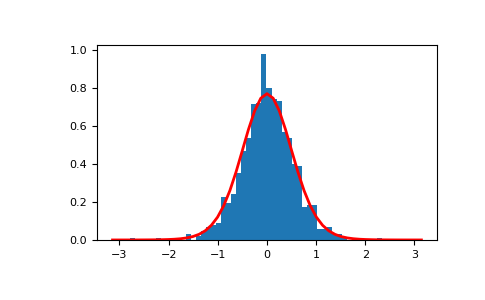
Display the histogram of the samples, along with the probability density function:

>>> import matplotlib.pyplot as plt
>>> from scipy.special import i0
>>> plt.hist(s, 50, normed=True)
>>> x = np.linspace(-np.pi, np.pi, num=51)
>>> y = np.exp(kappa*np.cos(x-mu))/(2*np.pi*i0(kappa))
>>> plt.plot(x, y, linewidth=2, color='r')
>>> plt.show()

(Source code, png, pdf)

../../_images/numpy-random-RandomState-vonmises-1.png