2.5.3. Linear System Solvers
sparse matrix/eigenvalue problem solvers live in
scipy.sparse.linalg- the submodules:
dsolve: direct factorization methods for solving linear systemsisolve: iterative methods for solving linear systemseigen: sparse eigenvalue problem solvers
all solvers are accessible from:
>>> import scipy.sparse.linalg as spla
>>> spla.__all__
['LinearOperator', 'Tester', 'arpack', 'aslinearoperator', 'bicg',
'bicgstab', 'cg', 'cgs', 'csc_matrix', 'csr_matrix', 'dsolve',
'eigen', 'eigen_symmetric', 'factorized', 'gmres', 'interface',
'isolve', 'iterative', 'lgmres', 'linsolve', 'lobpcg', 'lsqr',
'minres', 'np', 'qmr', 'speigs', 'spilu', 'splu', 'spsolve', 'svd',
'test', 'umfpack', 'use_solver', 'utils', 'warnings']
2.5.3.1. Sparse Direct Solvers
- default solver: SuperLU 4.0
- included in SciPy
- real and complex systems
- both single and double precision
- optional: umfpack
- real and complex systems
- double precision only
- recommended for performance
- wrappers now live in
scikits.umfpack - check-out the new
scikits.suitesparseby Nathaniel Smith
2.5.3.1.1. Examples
import the whole module, and see its docstring:
>>> from scipy.sparse.linalg import dsolve
>>> help(dsolve)
both superlu and umfpack can be used (if the latter is installed) as follows:
prepare a linear system:
>>> import numpy as np
>>> from scipy import sparse
>>> mtx = sparse.spdiags([[1, 2, 3, 4, 5], [6, 5, 8, 9, 10]], [0, 1], 5, 5)
>>> mtx.todense()
matrix([[ 1,  5,  0,  0,  0],
        [ 0,  2,  8,  0,  0],
        [ 0,  0,  3,  9,  0],
        [ 0,  0,  0,  4, 10],
        [ 0,  0,  0,  0,  5]])
>>> rhs = np.array([1, 2, 3, 4, 5], dtype=np.float32)
solve as single precision real:
>>> mtx1 = mtx.astype(np.float32)
>>> x = dsolve.spsolve(mtx1, rhs, use_umfpack=False)
>>> print(x)
[ 106.   -21.     5.5   -1.5    1. ]
>>> print("Error: %s" % (mtx1 * x - rhs))
Error:  [ 0.  0.  0.  0.  0.]
solve as double precision real:
>>> mtx2 = mtx.astype(np.float64)
>>> x = dsolve.spsolve(mtx2, rhs, use_umfpack=True)
>>> print(x)
[ 106.   -21.     5.5   -1.5    1. ]
>>> print("Error: %s" % (mtx2 * x - rhs))
Error:  [ 0.  0.  0.  0.  0.]
solve as single precision complex:
>>> mtx1 = mtx.astype(np.complex64)
>>> x = dsolve.spsolve(mtx1, rhs, use_umfpack=False)
>>> print(x)
[ 106.0+0.j  -21.0+0.j    5.5+0.j   -1.5+0.j    1.0+0.j]
>>> print("Error: %s" % (mtx1 * x - rhs))
Error:  [ 0.+0.j  0.+0.j  0.+0.j  0.+0.j  0.+0.j]
solve as double precision complex:
>>> mtx2 = mtx.astype(np.complex128)
>>> x = dsolve.spsolve(mtx2, rhs, use_umfpack=True)
>>> print(x)
[ 106.0+0.j  -21.0+0.j    5.5+0.j   -1.5+0.j    1.0+0.j]
>>> print("Error: %s" % (mtx2 * x - rhs))
Error:  [ 0.+0.j  0.+0.j  0.+0.j  0.+0.j  0.+0.j]
"""
Solve a linear system
=======================

Construct a 1000x1000 lil_matrix and add some values to it, convert it
to CSR format and solve A x = b for x:and solve a linear system with a
direct solver.
"""
import numpy as np
import scipy.sparse as sps
from matplotlib import pyplot as plt
from scipy.sparse.linalg.dsolve import linsolve

rand = np.random.rand

mtx = sps.lil_matrix((1000, 1000), dtype=np.float64)
mtx[0, :100] = rand(100)
mtx[1, 100:200] = mtx[0, :100]
mtx.setdiag(rand(1000))

plt.clf()
plt.spy(mtx, marker='.', markersize=2)
plt.show()

mtx = mtx.tocsr()
rhs = rand(1000)

x = linsolve.spsolve(mtx, rhs)

print('rezidual: %r' % np.linalg.norm(mtx * x - rhs))
2.5.3.2. Iterative Solvers
- the
isolvemodule contains the following solvers: bicg(BIConjugate Gradient)bicgstab(BIConjugate Gradient STABilized)cg(Conjugate Gradient) - symmetric positive definite matrices onlycgs(Conjugate Gradient Squared)gmres(Generalized Minimal RESidual)minres(MINimum RESidual)qmr(Quasi-Minimal Residual)
- the
2.5.3.2.1. Common Parameters
mandatory:
- A : {sparse matrix, dense matrix, LinearOperator}
The N-by-N matrix of the linear system.
- b : {array, matrix}
Right hand side of the linear system. Has shape (N,) or (N,1).
optional:
- x0 : {array, matrix}
Starting guess for the solution.
- tol : float
Relative tolerance to achieve before terminating.
- maxiter : integer
Maximum number of iterations. Iteration will stop after maxiter steps even if the specified tolerance has not been achieved.
- M : {sparse matrix, dense matrix, LinearOperator}
Preconditioner for A. The preconditioner should approximate the inverse of A. Effective preconditioning dramatically improves the rate of convergence, which implies that fewer iterations are needed to reach a given error tolerance.
- callback : function
User-supplied function to call after each iteration. It is called as callback(xk), where xk is the current solution vector.
2.5.3.2.2. LinearOperator Class
from scipy.sparse.linalg.interface import LinearOperator
- common interface for performing matrix vector products
- useful abstraction that enables using dense and sparse matrices within the solvers, as well as matrix-free solutions
- has shape and matvec() (+ some optional parameters)
- example:
>>> import numpy as np
>>> from scipy.sparse.linalg import LinearOperator
>>> def mv(v):
...     return np.array([2*v[0], 3*v[1]])
...
>>> A = LinearOperator((2, 2), matvec=mv)
>>> A
<2x2 LinearOperator with unspecified dtype>
>>> A.matvec(np.ones(2))
array([ 2.,  3.])
>>> A * np.ones(2)
array([ 2.,  3.])
2.5.3.2.3. A Few Notes on Preconditioning
- problem specific
- often hard to develop
- if not sure, try ILU
- available in
dsolveasspilu()
- available in
2.5.3.3. Eigenvalue Problem Solvers
2.5.3.3.1. The eigen module
arpack* a collection of Fortran77 subroutines designed to solve large scale eigenvalue problemslobpcg(Locally Optimal Block Preconditioned Conjugate Gradient Method) * works very well in combination with PyAMG * example by Nathan Bell:""" Compute eigenvectors and eigenvalues using a preconditioned eigensolver ======================================================================== In this example Smoothed Aggregation (SA) is used to precondition the LOBPCG eigensolver on a two-dimensional Poisson problem with Dirichlet boundary conditions. """ import scipy from scipy.sparse.linalg import lobpcg from pyamg import smoothed_aggregation_solver from pyamg.gallery import poisson N = 100 K = 9 A = poisson((N,N), format='csr') # create the AMG hierarchy ml = smoothed_aggregation_solver(A) # initial approximation to the K eigenvectors X = scipy.rand(A.shape[0], K) # preconditioner based on ml M = ml.aspreconditioner() # compute eigenvalues and eigenvectors with LOBPCG W,V = lobpcg(A, X, M=M, tol=1e-8, largest=False) #plot the eigenvectors import pylab pylab.figure(figsize=(9,9)) for i in range(K): pylab.subplot(3, 3, i+1) pylab.title('Eigenvector %d' % i) pylab.pcolor(V[:,i].reshape(N,N)) pylab.axis('equal') pylab.axis('off') pylab.show()
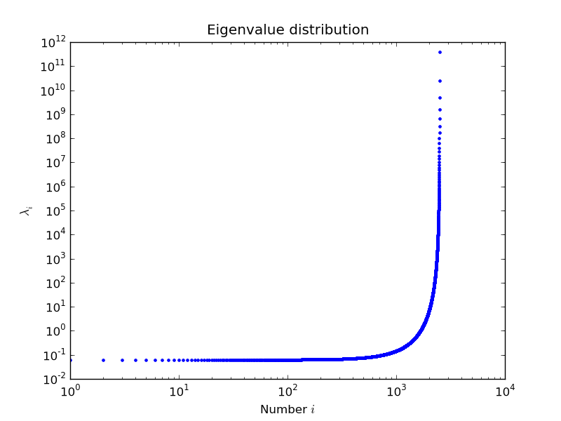
example by Nils Wagner:
output:
$ python examples/lobpcg_sakurai.py
Results by LOBPCG for n=2500

[ 0.06250083  0.06250028  0.06250007]

Exact eigenvalues

[ 0.06250005  0.0625002   0.06250044]

Elapsed time 7.01