
1.3.1. NumPy数组对象
Section contents
1.3.1.1. What are NumPy and NumPy arrays?
1.3.1.1.1. NumPy数组
| Python对象: |
|
|---|---|
| NumPy provides: |
|
>>> import numpy as np
>>> a = np.array([0, 1, 2, 3])
>>> a
array([0, 1, 2, 3])
For example, An array containing:
- values of an experiment/simulation at discrete time steps
- 由测量装置记录的信号,例如声波
- 图像的像素、灰度或颜色
- 3-D data measured at different X-Y-Z positions, e.g. MRI scan
- ...
Why it is useful: Memory-efficient container that provides fast numerical operations.
In [1]: L = range(1000)

In [2]: %timeit [i**2 for i in L]
1000 loops, best of 3: 403 us per loop

In [3]: a = np.arange(1000)

In [4]: %timeit a**2
100000 loops, best of 3: 12.7 us per loop
1.3.1.1.2. NumPy参考文档
交互式帮助:
In [5]: np.array?
String Form:<built-in function array>
Docstring:
array(object, dtype=None, copy=True, order=None, subok=False, ndmin=0, ...
查找某个东西:
>>> np.lookfor('create array')
Search results for 'create array'
---------------------------------
numpy.array
    Create an array.
numpy.memmap
    Create a memory-map to an array stored in a *binary* file on disk.
In [6]: np.con*?
np.concatenate
np.conj
np.conjugate
np.convolve
1.3.1.2. Creating arrays
1.3.1.2.1. 手动构建数组
1-D:
>>> a = np.array([0, 1, 2, 3])
>>> a
array([0, 1, 2, 3])
>>> a.ndim
1
>>> a.shape
(4,)
>>> len(a)
4
2-D, 3-D, ...:
>>> b = np.array([[0, 1, 2], [3, 4, 5]])    # 2 x 3 array
>>> b
array([[0, 1, 2],
       [3, 4, 5]])
>>> b.ndim
2
>>> b.shape
(2, 3)
>>> len(b)     # returns the size of the first dimension
2

>>> c = np.array([[[1], [2]], [[3], [4]]])
>>> c
array([[[1],
        [2]],

       [[3],
        [4]]])
>>> c.shape
(2, 2, 1)
Exercise: Simple arrays
- Create a simple two dimensional array. First, redo the examples from above. And then create your own: how about odd numbers counting backwards on the first row, and even numbers on the second?
- Use the functions
len(),numpy.shape()on these arrays. How do they relate to each other? 以及与数组的ndim属性的关系?
1.3.1.2.2. 创建数组的函数
在实践中,我们很少一个一个地输入元素...
Evenly spaced:
>>> a = np.arange(10) # 0 .. n-1  (!)
>>> a
array([0, 1, 2, 3, 4, 5, 6, 7, 8, 9])
>>> b = np.arange(1, 9, 2) # start, end (exclusive), step
>>> b
array([1, 3, 5, 7])
或按点的个数:
>>> c = np.linspace(0, 1, 6)   # start, end, num-points
>>> c
array([ 0. ,  0.2,  0.4,  0.6,  0.8,  1. ])
>>> d = np.linspace(0, 1, 5, endpoint=False)
>>> d
array([ 0. ,  0.2,  0.4,  0.6,  0.8])
常用数组:
>>> a = np.ones((3, 3))  # reminder: (3, 3) is a tuple
>>> a
array([[ 1.,  1.,  1.],
       [ 1.,  1.,  1.],
       [ 1.,  1.,  1.]])
>>> b = np.zeros((2, 2))
>>> b
array([[ 0.,  0.],
       [ 0.,  0.]])
>>> c = np.eye(3)
>>> c
array([[ 1.,  0.,  0.],
       [ 0.,  1.,  0.],
       [ 0.,  0.,  1.]])
>>> d = np.diag(np.array([1, 2, 3, 4]))
>>> d
array([[1, 0, 0, 0],
       [0, 2, 0, 0],
       [0, 0, 3, 0],
       [0, 0, 0, 4]])
np.random: random numbers (Mersenne Twister PRNG):>>> a = np.random.rand(4) # uniform in [0, 1] >>> a array([ 0.95799151, 0.14222247, 0.08777354, 0.51887998]) >>> b = np.random.randn(4) # Gaussian >>> b array([ 0.37544699, -0.11425369, -0.47616538, 1.79664113]) >>> np.random.seed(1234) # Setting the random seed
Exercise: Creating arrays using functions
- Experiment with
arange,linspace,ones,zeros,eyeanddiag. - Create different kinds of arrays with random numbers.
- Try setting the seed before creating an array with random values.
- Look at the function
np.empty. What does it do? When might this be useful?
1.3.1.3. Basic data types
你可能已经注意到,在某些情况下,数组元素显示有后面的点(例如2. vs 2)。This is due to a difference in the data-type used:
>>> a = np.array([1, 2, 3])
>>> a.dtype
dtype('int64')

>>> b = np.array([1., 2., 3.])
>>> b.dtype
dtype('float64')
Different data-types allow us to store data more compactly in memory, but most of the time we simply work with floating point numbers. Note that, in the example above, NumPy auto-detects the data-type from the input.
你可以显式指定所需的数据类型:
>>> c = np.array([1, 2, 3], dtype=float)
>>> c.dtype
dtype('float64')
The default data type is floating point:
>>> a = np.ones((3, 3))
>>> a.dtype
dtype('float64')
There are also other types:
| 复数: | >>> d = np.array([1+2j, 3+4j, 5+6*1j])
>>> d.dtype
dtype('complex128')
|
|---|---|
| Bool: | >>> e = np.array([True, False, False, True])
>>> e.dtype
dtype('bool')
|
| Strings: | >>> f = np.array(['Bonjour', 'Hello', 'Hallo',])
>>> f.dtype # <--- strings containing max. 7 letters
dtype('S7')
|
| 更多类型: |
|
1.3.1.4. 基本的可视化 
Now that we have our first data arrays, we are going to visualize them.
Start by launching IPython:
$ ipython
或者notebook:
$ ipython notebook
IPython启动之后,启用交互式画图:
>>> %matplotlib
或者,从notebook中,在notebook中启用画图:
>>> %matplotlib inline
inline对notebook很重要,这样图表显示在notebook中,而不是显示在新窗口中。
Matplotlib is a 2D plotting package. 我们可以如下导入其函数:
>>> import matplotlib.pyplot as plt # the tidy way
然后使用(请注意,如果你未使用%matplotlib启用交互图,则必须显式使用show):
>>> plt.plot(x, y)       # line plot
>>> plt.show()           # <-- shows the plot (not needed with interactive plots)
或者,如果你已启用%matplotlib的交互式画图:
>>> plt.plot(x, y) # line plot
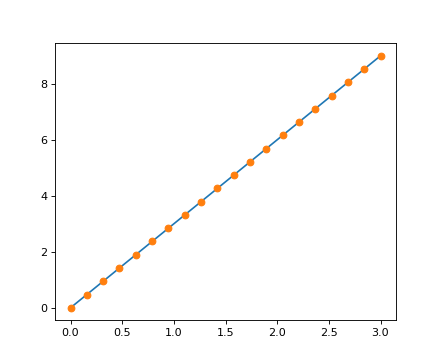
1D绘图:
>>> x = np.linspace(0, 3, 20)
>>> y = np.linspace(0, 9, 20)
>>> plt.plot(x, y)       # line plot
[<matplotlib.lines.Line2D object at ...>]
>>> plt.plot(x, y, 'o')  # dot plot
[<matplotlib.lines.Line2D object at ...>]
[source code, hires.png, pdf]
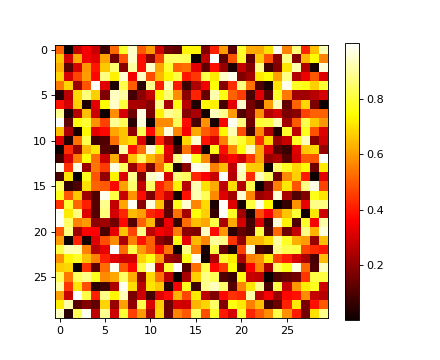
2D arrays (such as images):
>>> image = np.random.rand(30, 30)
>>> plt.imshow(image, cmap=plt.cm.hot)
>>> plt.colorbar()
<matplotlib.colorbar.Colorbar instance at ...>
[source code, hires.png, pdf]
See also
更多在:matplotlib一章
Exercise: Simple visualizations
- Plot some simple arrays: a cosine as a function of time and a 2D matrix.
- Try using the
graycolormap on the 2D matrix.
1.3.1.5. Indexing and slicing
可以按照与其他Python序列(例如列表)相同的方式访问和赋值数组的元素:
>>> a = np.arange(10)
>>> a
array([0, 1, 2, 3, 4, 5, 6, 7, 8, 9])
>>> a[0], a[2], a[-1]
(0, 2, 9)
Warning
指数从0开始,和其他Python序列(以及C/C++)一样。In contrast, in Fortran or Matlab, indices begin at 1.
支持反转python序列的通常写法:
>>> a[::-1]
array([9, 8, 7, 6, 5, 4, 3, 2, 1, 0])
对于多维数组,索引是整数组成的元组:
>>> a = np.diag(np.arange(3))
>>> a
array([[0, 0, 0],
       [0, 1, 0],
       [0, 0, 2]])
>>> a[1, 1]
1
>>> a[2, 1] = 10 # third line, second column
>>> a
array([[ 0,  0,  0],
       [ 0,  1,  0],
       [ 0, 10,  2]])
>>> a[1]
array([0, 1, 0])
Note
- In 2D, the first dimension corresponds to rows, the second to columns.
- 对于多维数组
a,a[0]解释为获取未指定的维度中的所有元素。
Slicing: Arrays, like other Python sequences can also be sliced:
>>> a = np.arange(10)
>>> a
array([0, 1, 2, 3, 4, 5, 6, 7, 8, 9])
>>> a[2:9:3] # [start:end:step]
array([2, 5, 8])
Note that the last index is not included! :
>>> a[:4]
array([0, 1, 2, 3])
不需要所有三个切片分量:默认情况下,start为0,end是最后一个,step为1:
>>> a[1:3]
array([1, 2])
>>> a[::2]
array([0, 2, 4, 6, 8])
>>> a[3:]
array([3, 4, 5, 6, 7, 8, 9])
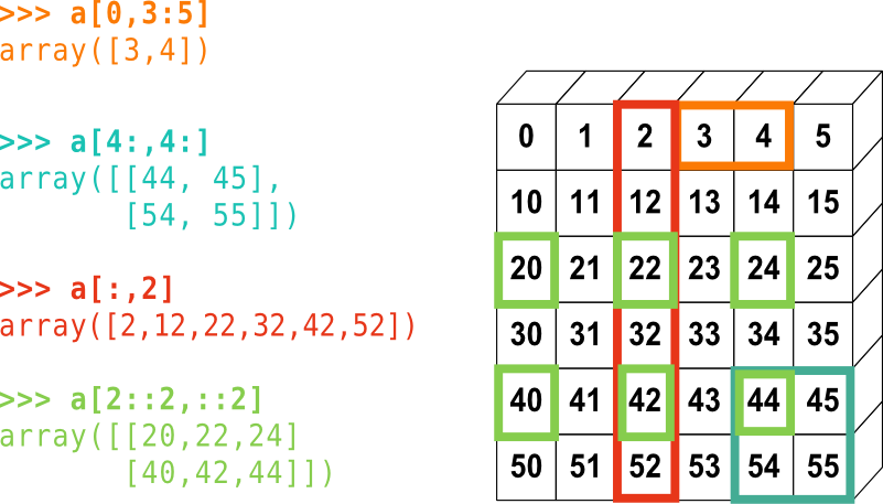
NumPy索引和切片摘要的小小图解...
你还可以组合赋值和切片:
>>> a = np.arange(10)
>>> a[5:] = 10
>>> a
array([ 0,  1,  2,  3,  4, 10, 10, 10, 10, 10])
>>> b = np.arange(5)
>>> a[5:] = b[::-1]
>>> a
array([0, 1, 2, 3, 4, 4, 3, 2, 1, 0])
Exercise: Indexing and slicing
尝试不同的切片风格,使用
start,end和step:从一个linspace开始,尝试获得从前向后数的奇数,和向后向前数的偶数。重复上图中的切片。你可以使用以下表达式创建数组:
>>> np.arange(6) + np.arange(0, 51, 10)[:, np.newaxis]
array([[ 0,  1,  2,  3,  4,  5],
       [10, 11, 12, 13, 14, 15],
       [20, 21, 22, 23, 24, 25],
       [30, 31, 32, 33, 34, 35],
       [40, 41, 42, 43, 44, 45],
       [50, 51, 52, 53, 54, 55]])
Exercise: Array creation
Create the following arrays (with correct data types):
[[1, 1, 1, 1],
 [1, 1, 1, 1],
 [1, 1, 1, 2],
 [1, 6, 1, 1]]

[[0., 0., 0., 0., 0.],
 [2., 0., 0., 0., 0.],
 [0., 3., 0., 0., 0.],
 [0., 0., 4., 0., 0.],
 [0., 0., 0., 5., 0.],
 [0., 0., 0., 0., 6.]]
课程标准:每个用3句话
提示:可以用类似于列表的方式访问各个数组元素,例如a[1]或a[1, 2]。
提示:查看diag的docstring。
练习:tile数组的创建
Skim through the documentation for np.tile, and use this function to construct the array:
[[4, 3, 4, 3, 4, 3],
 [2, 1, 2, 1, 2, 1],
 [4, 3, 4, 3, 4, 3],
 [2, 1, 2, 1, 2, 1]]
1.3.1.6. 拷贝和视图 
A slicing operation creates a view on the original array, which is just a way of accessing array data. Thus the original array is not copied in memory. 你可以使用np.may_share_memory()来检查两个数组是否共享同一个内存块。但请注意,这使用启发式算法,可能会给你假阳性。
When modifying the view, the original array is modified as well:
>>> a = np.arange(10)
>>> a
array([0, 1, 2, 3, 4, 5, 6, 7, 8, 9])
>>> b = a[::2]
>>> b
array([0, 2, 4, 6, 8])
>>> np.may_share_memory(a, b)
True
>>> b[0] = 12
>>> b
array([12,  2,  4,  6,  8])
>>> a   # (!)
array([12,  1,  2,  3,  4,  5,  6,  7,  8,  9])

>>> a = np.arange(10)
>>> c = a[::2].copy()  # force a copy
>>> c[0] = 12
>>> a
array([0, 1, 2, 3, 4, 5, 6, 7, 8, 9])

>>> np.may_share_memory(a, c)
False
这种行为第一次看到可能令人惊讶...但它节省内存和时间。
Worked example: Prime number sieve
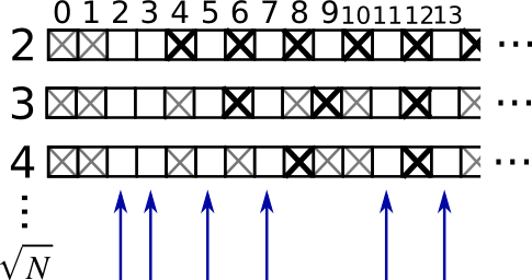
计算0-99之间的素数,用筛子
- 构造一个形状为(100,) 的布尔数组
is_prime,开始全部填充True:
>>> is_prime = np.ones((100,), dtype=bool)
- 叉掉0和1,它们不是素数:
>>> is_prime[:2] = 0
- 对于从2开始的每个整数
j,叉掉它的倍数:
>>> N_max = int(np.sqrt(len(is_prime) - 1))
>>> for j in range(2, N_max + 1):
...     is_prime[2*j::j] = False
浏览
help(np.nonzero),然后打印这些素数Follow-up:
- Move the above code into a script file named
prime_sieve.py - 运行它并检查它的工作
- Use the optimization suggested in the sieve of Eratosthenes:
- Skip
jwhich are already known to not be primes - 叉掉的第一个数字是

- Move the above code into a script file named
1.3.1.7. 花式索引 
NumPy数组不但可以用切片索引,而且可以用布尔数组或整数数组(掩码)索引。This method is called fancy indexing. 它创建拷贝而不是视图。
1.3.1.7.1. 使用布尔掩码
>>> np.random.seed(3)
>>> a = np.random.randint(0, 21, 15)
>>> a
array([10,  3,  8,  0, 19, 10, 11,  9, 10,  6,  0, 20, 12,  7, 14])
>>> (a % 3 == 0)
array([False,  True, False,  True, False, False, False,  True, False,
        True,  True, False,  True, False, False], dtype=bool)
>>> mask = (a % 3 == 0)
>>> extract_from_a = a[mask] # or,  a[a%3==0]
>>> extract_from_a           # extract a sub-array with the mask
array([ 3,  0,  9,  6,  0, 12])
Indexing with a mask can be very useful to assign a new value to a sub-array:
>>> a[a % 3 == 0] = -1
>>> a
array([10, -1,  8, -1, 19, 10, 11, -1, 10, -1, -1, 20, -1,  7, 14])
1.3.1.7.2. 用整数数组索引
>>> a = np.arange(0, 100, 10)
>>> a
array([ 0, 10, 20, 30, 40, 50, 60, 70, 80, 90])
Indexing can be done with an array of integers, where the same index is repeated several time:
>>> a[[2, 3, 2, 4, 2]]  # note: [2, 3, 2, 4, 2] is a Python list
array([20, 30, 20, 40, 20])
New values can be assigned with this kind of indexing:
>>> a[[9, 7]] = -100
>>> a
array([   0,   10,   20,   30,   40,   50,   60, -100,   80, -100])
When a new array is created by indexing with an array of integers, the new array has the same shape than the array of integers:
>>> a = np.arange(10)
>>> idx = np.array([[3, 4], [9, 7]])
>>> idx.shape
(2, 2)
>>> a[idx]
array([[3, 4],
       [9, 7]])
下面的图片说明了各种花式索引应用
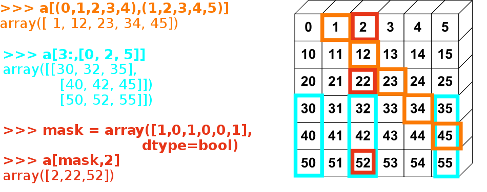
练习:花式索引
- 再次,再现上图中所示的花式索引。
- 在左边使用花式索引,右边使用数组创建将值赋值到数组,例如将上图中数组的一部分设置为零。