
1.3.2. 数组上的数值运算
Section contents
1.3.2.1. 元素级别运算 
1.3.2.1.1. 基本操作
标量:
>>> a = np.array([1, 2, 3, 4])
>>> a + 1
array([2, 3, 4, 5])
>>> 2**a
array([ 2,  4,  8, 16])
所有算术运算都是元素级别:
>>> b = np.ones(4) + 1
>>> a - b
array([-1.,  0.,  1.,  2.])
>>> a * b
array([ 2.,  4.,  6.,  8.])

>>> j = np.arange(5)
>>> 2**(j + 1) - j
array([ 2,  3,  6, 13, 28])
这些操作当然比你在纯python中做的更快:
>>> a = np.arange(10000)
>>> %timeit a + 1
10000 loops, best of 3: 24.3 us per loop
>>> l = range(10000)
>>> %timeit [i+1 for i in l]
1000 loops, best of 3: 861 us per loop
Warning
Array multiplication is not matrix multiplication:
>>> c = np.ones((3, 3))
>>> c * c                   # NOT matrix multiplication!
array([[ 1.,  1.,  1.],
       [ 1.,  1.,  1.],
       [ 1.,  1.,  1.]])
Note
Matrix multiplication:
>>> c.dot(c)
array([[ 3.,  3.,  3.],
       [ 3.,  3.,  3.],
       [ 3.,  3.,  3.]])
练习:元素级别运算
- 尝试简单的元素级别运算操作:将奇数元素和偶数元素相加
- 使用
%timeit来测试纯Python实现的时间。- Generate:
[2**0, 2**1, 2**2, 2**3, 2**4]a_j = 2^(3*j) - j
1.3.2.1.2. 其他操作
Comparisons:
>>> a = np.array([1, 2, 3, 4])
>>> b = np.array([4, 2, 2, 4])
>>> a == b
array([False,  True, False,  True], dtype=bool)
>>> a > b
array([False, False,  True, False], dtype=bool)
数组级别比较:
>>> a = np.array([1, 2, 3, 4])
>>> b = np.array([4, 2, 2, 4])
>>> c = np.array([1, 2, 3, 4])
>>> np.array_equal(a, b)
False
>>> np.array_equal(a, c)
True
Logical operations:
>>> a = np.array([1, 1, 0, 0], dtype=bool)
>>> b = np.array([1, 0, 1, 0], dtype=bool)
>>> np.logical_or(a, b)
array([ True,  True,  True, False], dtype=bool)
>>> np.logical_and(a, b)
array([ True, False, False, False], dtype=bool)
Transcendental函数:
>>> a = np.arange(5)
>>> np.sin(a)
array([ 0.        ,  0.84147098,  0.90929743,  0.14112001, -0.7568025 ])
>>> np.log(a)
array([       -inf,  0.        ,  0.69314718,  1.09861229,  1.38629436])
>>> np.exp(a)
array([  1.        ,   2.71828183,   7.3890561 ,  20.08553692,  54.59815003])
Shape mismatches
>>> a = np.arange(4)
>>> a + np.array([1, 2])
Traceback (most recent call last):
  File "<stdin>", line 1, in <module>
ValueError: operands could not be broadcast together with shapes (4) (2)
Broadcasting?我们稍后将回到这个问题。
转置:
>>> a = np.triu(np.ones((3, 3)), 1)   # see help(np.triu)
>>> a
array([[ 0.,  1.,  1.],
       [ 0.,  0.,  1.],
       [ 0.,  0.,  0.]])
>>> a.T
array([[ 0.,  0.,  0.],
       [ 1.,  0.,  0.],
       [ 1.,  1.,  0.]])
Warning
The transposition is a view
所以,以下代码是错误的,并且不会使矩阵对称:
>>> a += a.T
它对于小数组可以工作(因为缓冲),但是对于大数组将以不可预测的方式失败。
Note
Linear algebra
The sub-module numpy.linalg implements basic linear algebra, such as solving linear systems, singular value decomposition, etc. 但是,不能保证使用高效的例程对它进行编译,因此我们建议使用scipy.linalg,在线性代数运算:scipy.linalg中有详细讲述。
练习其他运算
- Look at the help for
np.allclose. 什么时候这可能用到?- Look at the help for
np.triuandnp.tril.
1.3.2.2. 基本的规约 
1.3.2.2.1. 计算和
>>> x = np.array([1, 2, 3, 4])
>>> np.sum(x)
10
>>> x.sum()
10
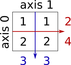
Sum by rows and by columns:
>>> x = np.array([[1, 1], [2, 2]])
>>> x
array([[1, 1],
       [2, 2]])
>>> x.sum(axis=0)   # columns (first dimension)
array([3, 3])
>>> x[:, 0].sum(), x[:, 1].sum()
(3, 3)
>>> x.sum(axis=1)   # rows (second dimension)
array([2, 4])
>>> x[0, :].sum(), x[1, :].sum()
(2, 4)
更高维度的思想相同:
>>> x = np.random.rand(2, 2, 2)
>>> x.sum(axis=2)[0, 1]
1.14764...
>>> x[0, 1, :].sum()
1.14764...
1.3.2.2.2. 其他规约
—— 工作方式相同(并接受axis=)
极值:
>>> x = np.array([1, 3, 2])
>>> x.min()
1
>>> x.max()
3

>>> x.argmin()  # index of minimum
0
>>> x.argmax()  # index of maximum
1
Logical operations:
>>> np.all([True, True, False])
False
>>> np.any([True, True, False])
True
Note
Can be used for array comparisons:
>>> a = np.zeros((100, 100))
>>> np.any(a != 0)
False
>>> np.all(a == a)
True

>>> a = np.array([1, 2, 3, 2])
>>> b = np.array([2, 2, 3, 2])
>>> c = np.array([6, 4, 4, 5])
>>> ((a <= b) & (b <= c)).all()
True
Statistics:
>>> x = np.array([1, 2, 3, 1])
>>> y = np.array([[1, 2, 3], [5, 6, 1]])
>>> x.mean()
1.75
>>> np.median(x)
1.5
>>> np.median(y, axis=-1) # last axis
array([ 2.,  5.])

>>> x.std()          # full population standard dev.
0.82915619758884995
...以及更多(最好是边往前边学习)。
练习:规约
- 假设有
sum,你期望看到什么其他函数?- What is the difference between
sumandcumsum?
Worked Example: data statistics
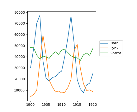
populations.txt中的数据描述了加拿大北部20年期间野兔和猞猁(和胡萝卜)的数量。
你可以在编辑器中查看数据,或者在IPython(shell和notebook)中查看数据:
In [1]: !cat data/populations.txt
First, load the data into a NumPy array:
>>> data = np.loadtxt('data/populations.txt')
>>> year, hares, lynxes, carrots = data.T  # trick: columns to variables
Then plot it:
>>> from matplotlib import pyplot as plt
>>> plt.axes([0.2, 0.1, 0.5, 0.8])
>>> plt.plot(year, hares, year, lynxes, year, carrots)
>>> plt.legend(('Hare', 'Lynx', 'Carrot'), loc=(1.05, 0.5))
[source code, hires.png, pdf]
随时间的种群平均数量:
>>> populations = data[:, 1:]
>>> populations.mean(axis=0)
array([ 34080.95238095,  20166.66666667,  42400.        ])
The sample standard deviations:
>>> populations.std(axis=0)
array([ 20897.90645809,  16254.59153691,   3322.50622558])
哪些物种每年有最高的种群数量?:
>>> np.argmax(populations, axis=1)
array([2, 2, 0, 0, 1, 1, 2, 2, 2, 2, 2, 2, 0, 0, 0, 1, 2, 2, 2, 2, 2])
工作示例:使用随机游走算法的扩散
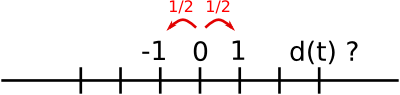
Let us consider a simple 1D random walk process: at each time step a walker jumps right or left with equal probability.
我们的兴趣在于找到一个随机游走者在t次向左或向右跳跃之后距原点的典型距离?我们将模拟许多“walker”找到这个规律,我们将使用数组计算技巧:我们将创建一个二维数组,用“stories”表示一个方向(每个步行者是一个story),时间表示另一个方向:

>>> n_stories = 1000 # number of walkers
>>> t_max = 200      # time during which we follow the walker
We randomly choose all the steps 1 or -1 of the walk:
>>> t = np.arange(t_max)
>>> steps = 2 * np.random.randint(0, 1 + 1, (n_stories, t_max)) - 1 # +1 because the high value is exclusive
>>> np.unique(steps) # Verification: all steps are 1 or -1
array([-1,  1])
我们通过随着时间的步数求和来建立距离:
>>> positions = np.cumsum(steps, axis=1) # axis = 1: dimension of time
>>> sq_distance = positions**2
We get the mean in the axis of the stories:
>>> mean_sq_distance = np.mean(sq_distance, axis=0)
Plot the results:
>>> plt.figure(figsize=(4, 3))
<matplotlib.figure.Figure object at ...>
>>> plt.plot(t, np.sqrt(mean_sq_distance), 'g.', t, np.sqrt(t), 'y-')
[<matplotlib.lines.Line2D object at ...>, <matplotlib.lines.Line2D object at ...>]
>>> plt.xlabel(r"$t$")
<matplotlib.text.Text object at ...>
>>> plt.ylabel(r"$\sqrt{\langle (\delta x)^2 \rangle}$")
<matplotlib.text.Text object at ...>
[source code, hires.png, pdf]

We find a well-known result in physics: the RMS distance grows as the square root of the time!
1.3.2.3. Broadcasting
numpy数组的基本运算(加法等)是元素级别的。This works on arrays of the same size.
然而,如果NumPy可以转换这些数组,使它们都具有相同的大小,那么也可以对不同大小的数组执行运算:这种转换称为broadcasting。
下图给出了broadcasting的示例:
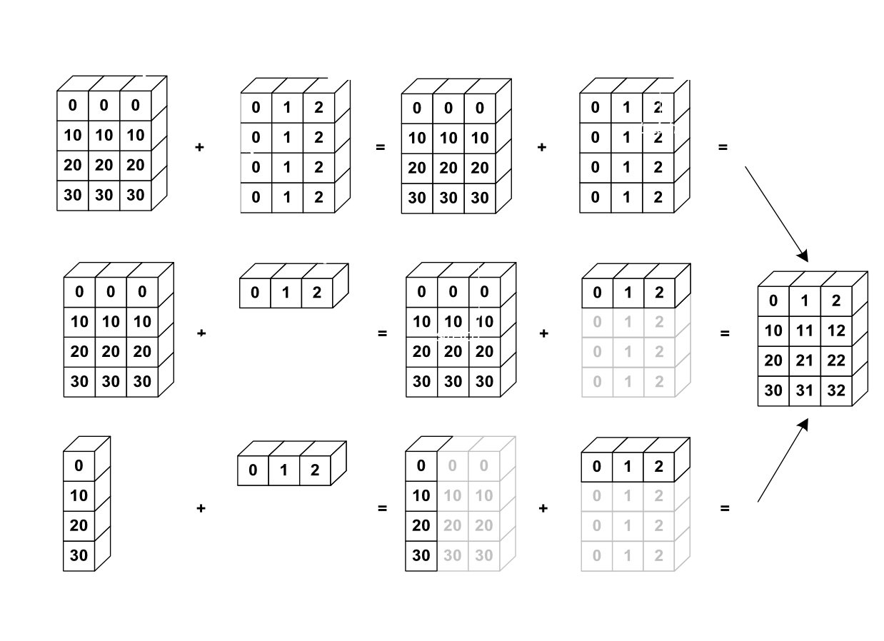
Let’s verify:
>>> a = np.tile(np.arange(0, 40, 10), (3, 1)).T
>>> a
array([[ 0,  0,  0],
       [10, 10, 10],
       [20, 20, 20],
       [30, 30, 30]])
>>> b = np.array([0, 1, 2])
>>> a + b
array([[ 0,  1,  2],
       [10, 11, 12],
       [20, 21, 22],
       [30, 31, 32]])
我们已经使用过broadcasting而并没有意识到它!:
>>> a = np.ones((4, 5))
>>> a[0] = 2  # we assign an array of dimension 0 to an array of dimension 1
>>> a
array([[ 2.,  2.,  2.,  2.,  2.],
       [ 1.,  1.,  1.,  1.,  1.],
       [ 1.,  1.,  1.,  1.,  1.],
       [ 1.,  1.,  1.,  1.,  1.]])
An useful trick:
>>> a = np.arange(0, 40, 10)
>>> a.shape
(4,)
>>> a = a[:, np.newaxis]  # adds a new axis -> 2D array
>>> a.shape
(4, 1)
>>> a
array([[ 0],
       [10],
       [20],
       [30]])
>>> a + b
array([[ 0,  1,  2],
       [10, 11, 12],
       [20, 21, 22],
       [30, 31, 32]])
Broadcasting看起来有点神奇,但是当我们想要解决一个问题,其输出数据是具有比输入数据更多维度的数组时,使用它是真的很自然。
工作示例:Broadcasting
Let’s construct an array of distances (in miles) between cities of Route 66: Chicago, Springfield, Saint-Louis, Tulsa, Oklahoma City, Amarillo, Santa Fe, Albuquerque, Flagstaff and Los Angeles.
>>> mileposts = np.array([0, 198, 303, 736, 871, 1175, 1475, 1544,
...        1913, 2448])
>>> distance_array = np.abs(mileposts - mileposts[:, np.newaxis])
>>> distance_array
array([[   0,  198,  303,  736,  871, 1175, 1475, 1544, 1913, 2448],
       [ 198,    0,  105,  538,  673,  977, 1277, 1346, 1715, 2250],
       [ 303,  105,    0,  433,  568,  872, 1172, 1241, 1610, 2145],
       [ 736,  538,  433,    0,  135,  439,  739,  808, 1177, 1712],
       [ 871,  673,  568,  135,    0,  304,  604,  673, 1042, 1577],
       [1175,  977,  872,  439,  304,    0,  300,  369,  738, 1273],
       [1475, 1277, 1172,  739,  604,  300,    0,   69,  438,  973],
       [1544, 1346, 1241,  808,  673,  369,   69,    0,  369,  904],
       [1913, 1715, 1610, 1177, 1042,  738,  438,  369,    0,  535],
       [2448, 2250, 2145, 1712, 1577, 1273,  973,  904,  535,    0]])

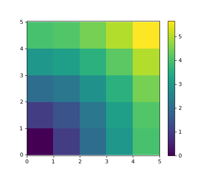
很多基于网格或基于网络的问题也可以使用broadcasting。例如,如果我们要计算从10x10网格上的点到原点的距离,我们可以这样做
>>> x, y = np.arange(5), np.arange(5)[:, np.newaxis]
>>> distance = np.sqrt(x ** 2 + y ** 2)
>>> distance
array([[ 0.        ,  1.        ,  2.        ,  3.        ,  4.        ],
       [ 1.        ,  1.41421356,  2.23606798,  3.16227766,  4.12310563],
       [ 2.        ,  2.23606798,  2.82842712,  3.60555128,  4.47213595],
       [ 3.        ,  3.16227766,  3.60555128,  4.24264069,  5.        ],
       [ 4.        ,  4.12310563,  4.47213595,  5.        ,  5.65685425]])
或用颜色表示:
>>> plt.pcolor(distance)
>>> plt.colorbar()
[source code, hires.png, pdf]
Remark : the numpy.ogrid function allows to directly create vectors x and y of the previous example, with two “significant dimensions”:
>>> x, y = np.ogrid[0:5, 0:5]
>>> x, y
(array([[0],
       [1],
       [2],
       [3],
       [4]]), array([[0, 1, 2, 3, 4]]))
>>> x.shape, y.shape
((5, 1), (1, 5))
>>> distance = np.sqrt(x ** 2 + y ** 2)
So, np.ogrid is very useful as soon as we have to handle computations on a grid. 另一方面,np.mgrid直接提供完整矩阵,用于我们不能(或不想)受益于broadcasting的情况:
>>> x, y = np.mgrid[0:4, 0:4]
>>> x
array([[0, 0, 0, 0],
       [1, 1, 1, 1],
       [2, 2, 2, 2],
       [3, 3, 3, 3]])
>>> y
array([[0, 1, 2, 3],
       [0, 1, 2, 3],
       [0, 1, 2, 3],
       [0, 1, 2, 3]])
1.3.2.4. Array shape manipulation
1.3.2.4.1. 平展
>>> a = np.array([[1, 2, 3], [4, 5, 6]])
>>> a.ravel()
array([1, 2, 3, 4, 5, 6])
>>> a.T
array([[1, 4],
       [2, 5],
       [3, 6]])
>>> a.T.ravel()
array([1, 4, 2, 5, 3, 6])
更高的维度:最后的维度“最先”解开。
1.3.2.4.2. 重塑形状
The inverse operation to flattening:
>>> a.shape
(2, 3)
>>> b = a.ravel()
>>> b = b.reshape((2, 3))
>>> b
array([[1, 2, 3],
       [4, 5, 6]])
或者,
>>> a.reshape((2, -1))    # unspecified (-1) value is inferred
array([[1, 2, 3],
       [4, 5, 6]])
Warning
ndarray.reshape 可能返回一个视图(参见help(np.reshape))也可能返回一个拷贝
>>> b[0, 0] = 99
>>> a
array([[99,  2,  3],
       [ 4,  5,  6]])
注意:reshape也可能会返回一个拷贝!:
>>> a = np.zeros((3, 2))
>>> b = a.T.reshape(3*2)
>>> b[0] = 9
>>> a
array([[ 0.,  0.],
       [ 0.,  0.],
       [ 0.,  0.]])
To understand this you need to learn more about the memory layout of a numpy array.
1.3.2.4.3. 添加维度
使用np.newaxis对象进行索引允许我们向数组添加一个轴(你已经在broadcasting部分看到过这一点):
>>> z = np.array([1, 2, 3])
>>> z
array([1, 2, 3])

>>> z[:, np.newaxis]
array([[1],
       [2],
       [3]])

>>> z[np.newaxis, :]
array([[1, 2, 3]])
1.3.2.4.4. 维度换位
>>> a = np.arange(4*3*2).reshape(4, 3, 2)
>>> a.shape
(4, 3, 2)
>>> a[0, 2, 1]
5
>>> b = a.transpose(1, 2, 0)
>>> b.shape
(3, 2, 4)
>>> b[2, 1, 0]
5
创建的也是一个视图:
>>> b[2, 1, 0] = -1
>>> a[0, 2, 1]
-1
1.3.2.4.5. 更改大小
Size of an array can be changed with ndarray.resize:
>>> a = np.arange(4)
>>> a.resize((8,))
>>> a
array([0, 1, 2, 3, 0, 0, 0, 0])
However, it must not be referred to somewhere else:
>>> b = a
>>> a.resize((4,))
Traceback (most recent call last):
  File "<stdin>", line 1, in <module>
ValueError: cannot resize an array that has been referenced or is
referencing another array in this way.  Use the resize function
Exercise: Shape manipulations
- 查看
reshape的文档字符串,尤其是注意事项部分,具有关于拷贝和视图的更多信息。 - Use
flattenas an alternative toravel. What is the difference? (Hint: check which one returns a view and which a copy) - 尝试使用
transpose进行维度换位。
1.3.2.5. Sorting data
沿某个轴排序:
>>> a = np.array([[4, 3, 5], [1, 2, 1]])
>>> b = np.sort(a, axis=1)
>>> b
array([[3, 4, 5],
       [1, 1, 2]])
Note
Sorts each row separately!
In-place sort:
>>> a.sort(axis=1)
>>> a
array([[3, 4, 5],
       [1, 1, 2]])
用花式索引排序:
>>> a = np.array([4, 3, 1, 2])
>>> j = np.argsort(a)
>>> j
array([2, 3, 1, 0])
>>> a[j]
array([1, 2, 3, 4])
Finding minima and maxima:
>>> a = np.array([4, 3, 1, 2])
>>> j_max = np.argmax(a)
>>> j_min = np.argmin(a)
>>> j_max, j_min
(0, 2)
Exercise: Sorting
- 尝试原位排序和异位排序。
- Try creating arrays with different dtypes and sorting them.
- Use
allorarray_equalto check the results.- 查看
np.random.shuffle,找到更快地创建可排序输入的方法。- 合并
ravel、sort和reshape。- Look at the
axiskeyword forsortand rewrite the previous exercise.
1.3.2.6. 小结 
需要知道什么才算入门?
Know how to create arrays :
array,arange,ones,zeros.Know the shape of the array with
array.shape, then use slicing to obtain different views of the array:array[::2], etc. Adjust the shape of the array usingreshapeor flatten it withravel.Obtain a subset of the elements of an array and/or modify their values with masks
>>> a[a < 0] = 0
Know miscellaneous operations on arrays, such as finding the mean or max (
array.max(),array.mean()). 不需要记住所有内容,而是要想到搜索文档(在线文档、help()、lookfor())!!对于高级应用:掌握整数数组的索引、以及broadcasting。Know more NumPy functions to handle various array operations.
Quick read
如果你想第一次快速通过Scipy讲义来学习生态系统,你可以直接跳到下一章:Matplotlib:画图。
本章的其余部分对于本简介的后面的内容不是必要的。但一定要回来完成这一章,以及做一些更多的练习。