
1.5. Scipy:高级科学计算
Authors: Adrien Chauve, Andre Espaze, Emmanuelle Gouillart, Gaël Varoquaux, Ralf Gommers
SciPy的
scipy软件包包含专用于科学计算中常见问题的各种工具箱。其不同的子模块对应于不同的应用,如插值、积分、优化、图像处理、统计、特殊功能等。
scipy可以与其他标准科学计算库进行比较,例如GSL(GNU Scientific Library for C and C++)或Matlab的工具箱。scipy是Python中用于科学计算程序的核心包;它的意图之一是有效地操作numpy数组,以便numpy和scipy可以同步工作。
在实现一个例程之前,值得检查所需的数据处理是否尚未在Scipy中实现。作为非专业程序员,科学家通常倾向于重新创造轮子,这会导致错误、非最佳、难以共享和无法维护的代码。By contrast, Scipy‘s routines are optimized and tested, and should therefore be used when possible.
章节内容
警告
本教程远非数值计算的介绍。因为列举scipy中不同的子模块和函数会很无聊,所以我们集中精力举几个例子来给出如何在科学计算中使用scipy的一般概念。
scipy由任务特定的子模块组成:
scipy.cluster |
矢量量化/Kmeans |
scipy.constants |
物理和数学常数 |
scipy.fftpack |
傅里叶变换 |
scipy.integrate |
集成例程 |
scipy.interpolate |
插值 |
scipy.io |
数据输入和输出 |
scipy.linalg |
线性代数例程 |
scipy.ndimage |
n维图像包 |
scipy.odr |
正交距离回归 |
scipy.optimize |
优化 |
scipy.signal |
信号处理 |
scipy.sparse |
稀疏矩阵 |
scipy.spatial |
空间数据结构和算法 |
scipy.special |
任何特殊的数学函数 |
scipy.stats |
统计 |
他们都依赖于numpy,但大多彼此独立。导入Numpy和这些Scipy模块的标准方式是:
>>> import numpy as np
>>> from scipy import stats  # same for other sub-modules
scipy主命名空间包含的函数大部分真实为numpy函数(试一下scipy.cos is np.cos)。它们暴露出来只是历史原因;通常没有理由在代码中使用import scipy。
1.5.1. 文件输入/输出: scipy.io 
加载和保存matlab文件:
>>> from scipy import io as spio
>>> a = np.ones((3, 3))
>>> spio.savemat('file.mat', {'a': a}) # savemat expects a dictionary
>>> data = spio.loadmat('file.mat', struct_as_record=True)
>>> data['a']
array([[ 1.,  1.,  1.],
       [ 1.,  1.,  1.],
       [ 1.,  1.,  1.]])
读取图片:
>>> from scipy import misc
>>> misc.imread('fname.png')
array(...)
>>> # Matplotlib also has a similar function
>>> import matplotlib.pyplot as plt
>>> plt.imread('fname.png')
array(...)
另见:
- 加载文本文件:
numpy.loadtxt()/numpy.savetxt()- 聪明加载text/csv文件:
numpy.genfromtxt()/numpy.recfromcsv()- 快速高效、但是是numpy特定的二进制格式:
numpy.save()/numpy.load()
1.5.2. 特殊函数: scipy.special 
特殊的函数是超越数函数。scipy.special模块的文档字符串编写得很好,所以我们不会在这里列出所有函数。常用的是:
- 贝塞尔函数,如
scipy.special.jn()(第n个整数阶Bessel函数)- 椭圆函数(
scipy.special.ellipj()用于雅可比椭圆函数,...)- 伽马函数:
scipy.special.gamma(),还要注意scipy.special.gammaln(),它将Gamma的log值赋予更高的数值精度。- Erf,高斯曲线下方的面积:
scipy.special.erf()
1.5.3. Linear algebra operations: scipy.linalg
scipy.linalg模块提供了标准的线性代数运算,依赖于基础的高效实现(BLAS,LAPACK)。
scipy.linalg.det()函数计算方阵的行列式:>>> from scipy import linalg >>> arr = np.array([[1, 2], ... [3, 4]]) >>> linalg.det(arr) -2.0 >>> arr = np.array([[3, 2], ... [6, 4]]) >>> linalg.det(arr) 0.0 >>> linalg.det(np.ones((3, 4))) Traceback (most recent call last): ... ValueError: expected square matrix
scipy.linalg.inv()函数计算方阵的倒数:>>> arr = np.array([[1, 2], ... [3, 4]]) >>> iarr = linalg.inv(arr) >>> iarr array([[-2. , 1. ], [ 1.5, -0.5]]) >>> np.allclose(np.dot(arr, iarr), np.eye(2)) True
最后计算一个奇异矩阵(它的行列式为零)的逆将会引起
LinAlgError:>>> arr = np.array([[3, 2], ... [6, 4]]) >>> linalg.inv(arr) Traceback (most recent call last): ... ...LinAlgError: singular matrix
还有更高级的操作,例如奇异值分解(SVD):
>>> arr = np.arange(9).reshape((3, 3)) + np.diag([1, 0, 1])
>>> uarr, spec, vharr = linalg.svd(arr)
得到的阵列频谱是:
>>> spec
array([ 14.88982544,   0.45294236,   0.29654967])
原始矩阵可以通过
svd与np.dot的输出的矩阵相乘来重新组合:>>> sarr = np.diag(spec) >>> svd_mat = uarr.dot(sarr).dot(vharr) >>> np.allclose(svd_mat, arr) True
SVD常用于统计和信号处理。
scipy.linalg中提供了许多其他标准分解(QR,LU,Cholesky,Schur)以及线性系统的求解器。
1.5.4. 快速傅立叶变换: scipy.fftpack 
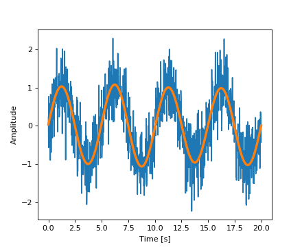
scipy.fftpack模块允许计算快速傅立叶变换。举例来说,一个(嘈杂的)输入信号可能看起来像:
>>> time_step = 0.02
>>> period = 5.
>>> time_vec = np.arange(0, 20, time_step)
>>> sig = np.sin(2 * np.pi / period * time_vec) + \
...       0.5 * np.random.randn(time_vec.size)
观察者不知道信号频率,只知道信号的采样时间步长sig。信号应该来自实际函数,所以傅里叶变换将是对称的。The scipy.fftpack.fftfreq() function will generate the sampling frequencies and scipy.fftpack.fft() will compute the fast Fourier transform:
>>> from scipy import fftpack
>>> sample_freq = fftpack.fftfreq(sig.size, d=time_step)
>>> sig_fft = fftpack.fft(sig)
由于得到的功率是对称的,因此只有频谱的正极部分需要用于查找频率:
>>> pidxs = np.where(sample_freq > 0)
>>> freqs = sample_freq[pidxs]
>>> power = np.abs(sig_fft)[pidxs]
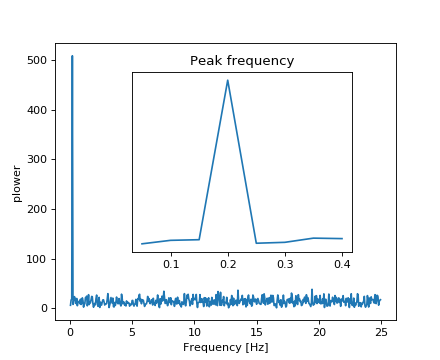
信号频率可以通过以下方式找到:
>>> freq = freqs[power.argmax()]
>>> np.allclose(freq, 1./period)  # check that correct freq is found
True
现在,高频噪声将从傅里叶变换信号中消除:
>>> sig_fft[np.abs(sample_freq) > freq] = 0
得到的滤波信号可以通过scipy.fftpack.ifft()函数进行计算:
>>> main_sig = fftpack.ifft(sig_fft)
结果可以通过以下方式查看:
>>> import pylab as plt
>>> plt.figure()
<matplotlib.figure.Figure object at 0x...>
>>> plt.plot(time_vec, sig)
[<matplotlib.lines.Line2D object at 0x...>]
>>> plt.plot(time_vec, main_sig, linewidth=3)
[<matplotlib.lines.Line2D object at 0x...>]
>>> plt.xlabel('Time [s]')
<matplotlib.text.Text object at 0x...>
>>> plt.ylabel('Amplitude')
<matplotlib.text.Text object at 0x...>
numpy.fft T0>
Numpy还具有FFT(numpy.fft)的实现。但是,通常scipy应该是首选的,因为它使用更高效的底层实现。
练习:消除月亮着陆图像
- 检查提供的图像moonlanding.png,它受到周期性噪音的严重污染。在本练习中,我们旨在使用快速傅立叶变换来清除噪音。
- 使用
pylab.imread()加载图像。 - 在
scipy.fftpack中查找并使用2-D FFT函数,并绘制图像的光谱(傅立叶变换)。您是否在查看频谱时遇到任何问题?如果是这样,为什么? - 频谱由高频和低频分量组成。噪声包含在频谱的高频部分,因此将其中一些分量设置为零(使用阵列分片)。
- 应用傅里叶逆变换来查看结果图像。
1.5.5. 优化和拟合: scipy.optimize 
优化是找到最小化或相等的数值解的问题。
scipy.optimize模块为函数最小化(标量或多维),曲线拟合和根发现提供了有用的算法。
>>> from scipy import optimize
寻找标量函数的最小值
我们来定义下面的函数:
>>> def f(x):
...     return x**2 + 10*np.sin(x)
并绘制它:
>>> x = np.arange(-10, 10, 0.1)
>>> plt.plot(x, f(x))
>>> plt.show()
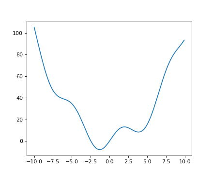
该函数的全局最小值约为-1.3,局部最小值约为3.8。
找到这个函数的最小值的一般和有效的方法是从给定的初始点开始进行梯度下降。BFGS算法是这样做的好方法:
>>> optimize.fmin_bfgs(f, 0)
Optimization terminated successfully.
         Current function value: -7.945823
         Iterations: 5
         Function evaluations: 24
         Gradient evaluations: 8
array([-1.30644003])
这种方法的一个可能的问题是,如果函数具有局部最小值,则算法可以根据初始点找到这些局部最小值而不是全局最小值:
>>> optimize.fmin_bfgs(f, 3, disp=0)
array([ 3.83746663])
如果我们不知道全局最小值的邻域选择初始点,我们需要求助于更昂贵的全局优化。为了找到全局最小值,我们使用scipy.optimize.basinhopping()(它将本地优化程序与本地优化程序的起点的随机抽样相结合):
版本0.12.0新增:在Scipy 0.12.0版本中增加了流动购物
>>> optimize.basinhopping(f, 0)
                  nfev: 1725
 minimization_failures: 0
                   fun: -7.9458233756152845
                     x: array([-1.30644001])
               message: ['requested number of basinhopping iterations completed successfully']
                  njev: 575
                   nit: 100
Another available (but much less efficient) global optimizer is scipy.optimize.brute() (brute force optimization on a grid). 针对不同类别的全局优化问题存在更高效的算法,但这超出了scipy的范围。一些有用的全局优化包是OpenOpt,IPOPT,PyGMO和PyEvolve。
注意
scipy用于包含例程anneal,它已从SciPy 0.14.0开始弃用,并在SciPy 0.16.0中删除。
To find the local minimum, let’s constraint the variable to the interval (0, 10) using scipy.optimize.fminbound():
>>> xmin_local = optimize.fminbound(f, 0, 10)
>>> xmin_local
3.8374671...
注意
在高级章节中更详细地讨论函数最小值的讨论:Mathematical optimization: finding minima of functions。
找到标量函数的根
要找到上面函数 的一个根,即
 的一个点,我们可以使用例如
scipy.optimize.fsolve():
>>> root = optimize.fsolve(f, 1)  # our initial guess is 1
>>> root
array([ 0.])
请注意,只有一个根被找到。检查的图表显示第二个根在-2.5附近。我们通过调整我们的初始猜测来找到它的确切值:
>>> root2 = optimize.fsolve(f, -2.5)
>>> root2
array([-2.47948183])
曲线拟合
假设我们从采样了一些噪音的数据:
>>> xdata = np.linspace(-10, 10, num=20)
>>> ydata = f(xdata) + np.random.randn(xdata.size)
现在,如果我们知道从中抽取样本的函数的函数形式(在这种情况下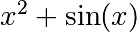 ),但不知道这些项的幅度,我们可以通过最小二乘法曲线拟合找到那些函数形式。首先,我们必须定义适合的函数:
>>> def f2(x, a, b):
...     return a*x**2 + b*np.sin(x)
然后我们可以使用scipy.optimize.curve_fit()来查找 和
和 :
:
>>> guess = [2, 2]
>>> params, params_covariance = optimize.curve_fit(f2, xdata, ydata, guess)
>>> params
array([  0.99667386,  10.17808313])
现在我们已经找到了f的最小值和根,并且使用了曲线拟合,我们将所有这些结果放在一个图中:
注意
在Scipy> = 0.11中,提供了所有最小化和根查找算法的统一接口:scipy.optimize.minimize(),scipy.optimize.minimize_scalar()和scipy.optimize.root()它们允许通过method关键字轻松比较各种算法。
您可以在scipy.optimize中找到与多维问题具有相同功能的算法。
练习:温度数据的曲线拟合
从1月份开始,阿拉斯加每月的极端温度由(以摄氏度计)给出:
max:  17,  19,  21,  28,  33,  38, 37,  37,  31,  23,  19,  18
min: -62, -59, -56, -46, -32, -18, -9, -13, -25, -46, -52, -58
- 绘制这些极端温度。
- 定义一个可以描述最小和最大温度的函数。提示:此功能必须有1年的时间。提示:包含时间偏移量。
- 使用
scipy.optimize.curve_fit()将此函数适用于数据。- 绘制结果。合适吗?如果不是,为什么?
- 最小和最大温度的时间偏差在拟合精度内是否相同?
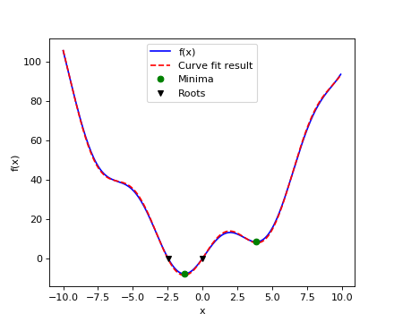
练习:2-D最小化
六驼驼驼背功能
有多个全球和当地最低标准。找到这个函数的全局最小值。
提示:
- 变量可以限制为
和
。
- 使用
numpy.meshgrid()和pylab.imshow()来直观地查找区域。- 使用
scipy.optimize.fmin_bfgs()或其他多维最小化程序。那里有多少个全球最低标准?这些点的功能价值是多少?初始猜测
会发生什么?
请参阅Non linear least squares curve fitting: application to point extraction in topographical lidar data以获得另一个更高级的示例。
1.5.6. 统计和随机数字: scipy.stats 
模块scipy.stats包含随机过程的统计工具和概率描述。用于各种随机过程的随机数生成器可以在numpy.random中找到。
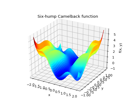
1.5.6.1. 直方图和概率密度函数
给定对随机过程的观察,它们的直方图是随机过程的PDF(概率密度函数)的估计量:
>>> a = np.random.normal(size=1000)
>>> bins = np.arange(-4, 5)
>>> bins
array([-4, -3, -2, -1,  0,  1,  2,  3,  4])
>>> histogram = np.histogram(a, bins=bins, normed=True)[0]
>>> bins = 0.5*(bins[1:] + bins[:-1])
>>> bins
array([-3.5, -2.5, -1.5, -0.5,  0.5,  1.5,  2.5,  3.5])
>>> from scipy import stats
>>> b = stats.norm.pdf(bins)  # norm is a distribution

>>> plt.plot(bins, histogram)
[<matplotlib.lines.Line2D object at ...>]
>>> plt.plot(bins, b)
[<matplotlib.lines.Line2D object at ...>]
如果我们知道随机过程属于给定的随机过程族,如正态过程,我们可以对观测值进行最大似然拟合,以估计基础分布的参数。在这里,我们对观测数据进行正常处理:
>>> loc, std = stats.norm.fit(a)
>>> loc
0.0314345570...
>>> std
0.9778613090...
练习:概率分布
从形状参数为1的伽玛分布生成1000个随机变量,然后绘制这些样本的直方图。你可以在上面绘制PDF(它应该匹配)?
额外:发行版有许多有用的方法。通过阅读文档字符串或使用IPython选项卡完成来探索它们。你可以通过在随机变量上使用fit方法找到1的形状参数吗?
1.5.6.2. 百分¶ T0>
中位数是以下一半观测值的数值,高于一半:
>>> np.median(a)
0.04041769593...
它也被称为百分位数50,因为50%的观察值低于它:
>>> stats.scoreatpercentile(a, 50)
0.0404176959...
同样,我们可以计算百分比90:
>>> stats.scoreatpercentile(a, 90)
1.3185699120...
百分位数是CDF的估计量:累积分布函数。
1.5.6.3. 统计测试
统计测试是一个决策指标。例如,如果我们有两组观测值,我们假设它们是由高斯过程产生的,那么我们可以使用一个T检验来确定这两组观测值是否有显着差异:
>>> a = np.random.normal(0, 1, size=100)
>>> b = np.random.normal(1, 1, size=10)
>>> stats.ttest_ind(a, b)
(array(-3.177574054...), 0.0019370639...)
结果输出由以下部分组成:
- T统计值:它是一个数字,其符号与两个随机过程之间的差异成正比,幅度与这种差异的显着性有关。
- p值:两个过程相同的概率。如果它接近1,那么这两个过程几乎肯定是相同的。它越接近零,这个过程就越有可能有不同的方法。
另见
关于statistics的章节介绍了更多精心制作的工具,用于统计测试和统计数据加载以及scipy之外的可视化。
1.5.7. 插值: scipy.interpolate 
scipy.interpolate对于拟合来自实验数据的函数是有用的,从而评估没有度量存在的点。该模块基于来自netlib项目的FITPACK Fortran子例程。
通过想象实验数据接近正弦函数:
>>> measured_time = np.linspace(0, 1, 10)
>>> noise = (np.random.random(10)*2 - 1) * 1e-1
>>> measures = np.sin(2 * np.pi * measured_time) + noise
scipy.interpolate.interp1d类可以构建一个线性插值函数:
>>> from scipy.interpolate import interp1d
>>> linear_interp = interp1d(measured_time, measures)
然后需要在感兴趣的时候评估scipy.interpolate.linear_interp实例:
>>> computed_time = np.linspace(0, 1, 50)
>>> linear_results = linear_interp(computed_time)
也可以通过提供kind可选关键字参数来选择三次插值:
>>> cubic_interp = interp1d(measured_time, measures, kind='cubic')
>>> cubic_results = cubic_interp(computed_time)
结果现在汇集在以下Matplotlib图中:
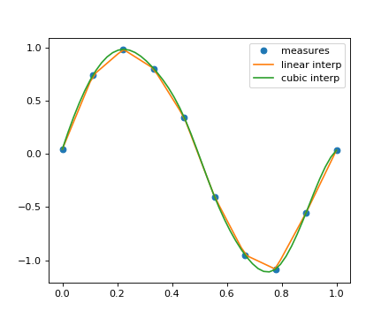
scipy.interpolate.interp2d类似于scipy.interpolate.interp1d,但是对于二维数组。请注意,对于interp系列,计算的时间必须保持在测量的时间范围内。参见Maximum wind speed prediction at the Sprogø station的摘要练习,以获得更高级的样条插值示例。
1.5.8. 数值积分: scipy.integrate 
最通用的集成例程是scipy.integrate.quad():
>>> from scipy.integrate import quad
>>> res, err = quad(np.sin, 0, np.pi/2)
>>> np.allclose(res, 1)
True
>>> np.allclose(err, 1 - res)
True
其他的集成方案可用于fixed_quad,quadrature,romberg。
scipy.integrate还具有集成常微分方程(ODE)的例程。In particular, scipy.integrate.odeint() is a general-purpose integrator using LSODA (Livermore Solver for Ordinary Differential equations with Automatic method switching for stiff and non-stiff problems), see the ODEPACK Fortran library for more details.
odeint solves first-order ODE systems of the form:
dy/dt = rhs(y1, y2, .., t0,...)
作为介绍,让我们解决 之间的ODE
  ,初始条件
,初始条件 。首先需要定义计算位置导数的函数:
>>> def calc_derivative(ypos, time, counter_arr):
...     counter_arr += 1
...     return -2 * ypos
...
添加了一个额外的参数counter_arr以说明可以在单个时间步骤内多次调用该函数,直到求解器收敛。计数器阵列定义为:
>>> counter = np.zeros((1,), dtype=np.uint16)
现在将计算轨迹:
>>> from scipy.integrate import odeint
>>> time_vec = np.linspace(0, 4, 40)
>>> yvec, info = odeint(calc_derivative, 1, time_vec,
...                     args=(counter,), full_output=True)
因此,派生函数被称为超过40次(这是时间步数):
>>> counter
array([129], dtype=uint16)
并且对于10个第一时间步骤中的每一个的迭代的累积次数可以通过以下获得:
>>> info['nfe'][:10]
array([31, 35, 43, 49, 53, 57, 59, 63, 65, 69], dtype=int32)
请注意,求解器在第一个步骤中需要更多的迭代。现在可以绘制轨迹的解决方案yvec:

scipy.integrate.odeint()的另一个例子是阻尼弹簧质量振荡器(二阶振荡器)。The position of a mass attached to a spring obeys the 2nd order ODE 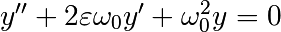 with
with  with
with  the spring constant,
  the mass and
  with
with  the damping coefficient. 对于这个例子,我们选择参数为:
>>> mass = 0.5  # kg
>>> kspring = 4  # N/m
>>> cviscous = 0.4  # N s/m
所以系统会被阻尼,因为:
>>> eps = cviscous / (2 * mass * np.sqrt(kspring/mass))
>>> eps < 1
True
对于scipy.integrate.odeint()求解器,二阶方程需要在两个一阶方程组的系统中针对向量 进行变换。定义
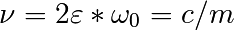 和
和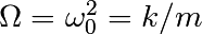 会很方便:
会很方便:
>>> nu_coef = cviscous / mass  # nu
>>> om_coef = kspring / mass  # Omega
因此,该功能将通过以下方式计算速度和加速度:
>>> def calc_deri(yvec, time, nu, om):
...     return (yvec[1], -nu * yvec[1] - om * yvec[0])
...
>>> time_vec = np.linspace(0, 10, 100)
>>> yinit = (1, 0)
>>> yarr = odeint(calc_deri, yinit, time_vec, args=(nu_coef, om_coef))
最终位置和速度显示在以下Matplotlib图中:
这两个例子只是常微分方程(ODE)。但是,Scipy中没有偏微分方程(PDE)求解器。一些用于解决PDE的Python包可用,如fipy或SfePy。
1.5.9. 信号处理: scipy.signal 
>>> from scipy import signal
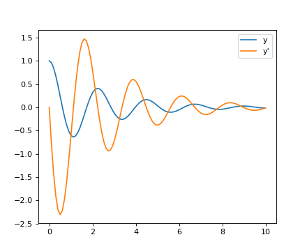
scipy.signal.detrend():从信号中移除线性趋势:>>> t = np.linspace(0, 5, 100) >>> x = t + np.random.normal(size=100) >>> plt.plot(t, x, linewidth=3) [<matplotlib.lines.Line2D object at ...>] >>> plt.plot(t, signal.detrend(x), linewidth=3) [<matplotlib.lines.Line2D object at ...>]
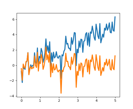
scipy.signal.resample():使用FFT将信号重采样到n点。>>> t = np.linspace(0, 5, 100) >>> x = np.sin(t) >>> plt.plot(t, x, linewidth=3) [<matplotlib.lines.Line2D object at ...>] >>> plt.plot(t[::2], signal.resample(x, 50), 'ko') [<matplotlib.lines.Line2D object at ...>]
scipy.signalhas many window functions:scipy.signal.hamming(),scipy.signal.bartlett(),scipy.signal.blackman()...scipy.signalhas filtering (median filterscipy.signal.medfilt(), Wienerscipy.signal.wiener()), but we will discuss this in the image section.
1.5.10. 图像处理: scipy.ndimage 
The submodule dedicated to image processing in scipy is scipy.ndimage.
>>> from scipy import ndimage
图像处理例程可以根据它们执行的处理的类别进行排序。
1.5.10.1. 对图像进行几何变换
改变方向,分辨率,..
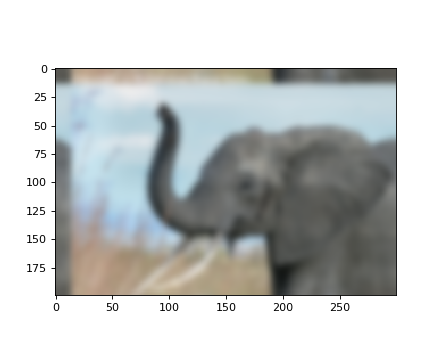
>>> from scipy import misc
>>> face = misc.face(gray=True)
>>> shifted_face = ndimage.shift(face, (50, 50))
>>> shifted_face2 = ndimage.shift(face, (50, 50), mode='nearest')
>>> rotated_face = ndimage.rotate(face, 30)
>>> cropped_face = face[50:-50, 50:-50]
>>> zoomed_face = ndimage.zoom(face, 2)
>>> zoomed_face.shape
(1536, 2048)
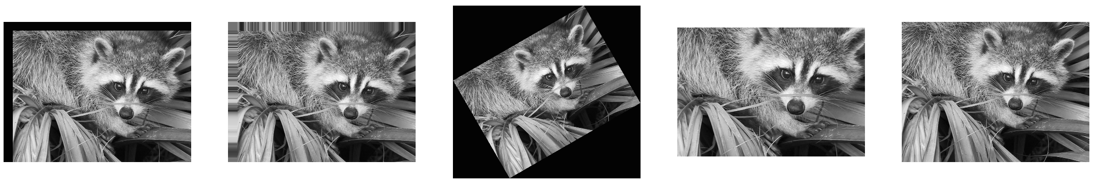
>>> plt.subplot(151)
<matplotlib.axes._subplots.AxesSubplot object at 0x...>

>>> plt.imshow(shifted_face, cmap=plt.cm.gray)
<matplotlib.image.AxesImage object at 0x...>

>>> plt.axis('off')
(-0.5, 1023.5, 767.5, -0.5)

>>> # etc.
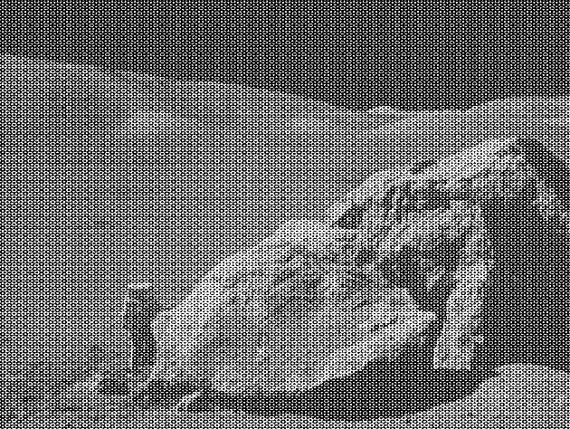
1.5.10.2. 图片过滤
>>> from scipy import misc
>>> face = misc.face(gray=True)
>>> face = face[:512, -512:]  # crop out square on right
>>> import numpy as np
>>> noisy_face = np.copy(face).astype(np.float)
>>> noisy_face += face.std() * 0.5 * np.random.standard_normal(face.shape)
>>> blurred_face = ndimage.gaussian_filter(noisy_face, sigma=3)
>>> median_face = ndimage.median_filter(noisy_face, size=5)
>>> from scipy import signal
>>> wiener_face = signal.wiener(noisy_face, (5, 5))

scipy.ndimage.filters和scipy.signal中的许多其他滤镜可应用于图像。
行使
比较不同过滤图像的直方图。
1.5.10.3. 数学形态学
数学形态学是一个源于集合论的数学理论。它表征和转换几何结构。二进制(黑色和白色)图像,尤其是可以使用这个理论进行变换:要变换的集合是相邻的非零值像素的集合。该理论还扩展到灰度图像。
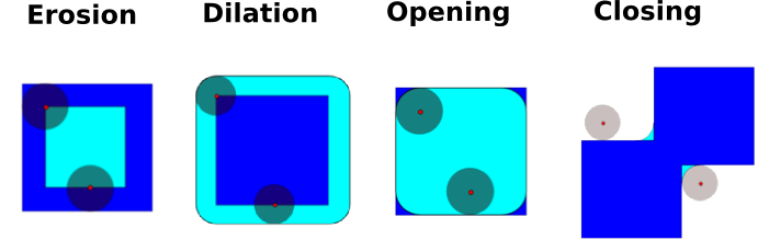
基本的数学形态学操作使用结构元素来修改其他几何结构。
让我们首先生成一个结构化元素
>>> el = ndimage.generate_binary_structure(2, 1)
>>> el
array([[False, True, False],
       [...True, True, True],
       [False, True, False]], dtype=bool)
>>> el.astype(np.int)
array([[0, 1, 0],
       [1, 1, 1],
       [0, 1, 0]])
侵蚀 T0>
>>> a = np.zeros((7, 7), dtype=np.int)
>>> a[1:6, 2:5] = 1
>>> a
array([[0, 0, 0, 0, 0, 0, 0],
       [0, 0, 1, 1, 1, 0, 0],
       [0, 0, 1, 1, 1, 0, 0],
       [0, 0, 1, 1, 1, 0, 0],
       [0, 0, 1, 1, 1, 0, 0],
       [0, 0, 1, 1, 1, 0, 0],
       [0, 0, 0, 0, 0, 0, 0]])
>>> ndimage.binary_erosion(a).astype(a.dtype)
array([[0, 0, 0, 0, 0, 0, 0],
       [0, 0, 0, 0, 0, 0, 0],
       [0, 0, 0, 1, 0, 0, 0],
       [0, 0, 0, 1, 0, 0, 0],
       [0, 0, 0, 1, 0, 0, 0],
       [0, 0, 0, 0, 0, 0, 0],
       [0, 0, 0, 0, 0, 0, 0]])
>>> #Erosion removes objects smaller than the structure
>>> ndimage.binary_erosion(a, structure=np.ones((5,5))).astype(a.dtype)
array([[0, 0, 0, 0, 0, 0, 0],
       [0, 0, 0, 0, 0, 0, 0],
       [0, 0, 0, 0, 0, 0, 0],
       [0, 0, 0, 0, 0, 0, 0],
       [0, 0, 0, 0, 0, 0, 0],
       [0, 0, 0, 0, 0, 0, 0],
       [0, 0, 0, 0, 0, 0, 0]])
扩张 T0>
>>> a = np.zeros((5, 5))
>>> a[2, 2] = 1
>>> a
array([[ 0.,  0.,  0.,  0.,  0.],
       [ 0.,  0.,  0.,  0.,  0.],
       [ 0.,  0.,  1.,  0.,  0.],
       [ 0.,  0.,  0.,  0.,  0.],
       [ 0.,  0.,  0.,  0.,  0.]])
>>> ndimage.binary_dilation(a).astype(a.dtype)
array([[ 0.,  0.,  0.,  0.,  0.],
       [ 0.,  0.,  1.,  0.,  0.],
       [ 0.,  1.,  1.,  1.,  0.],
       [ 0.,  0.,  1.,  0.,  0.],
       [ 0.,  0.,  0.,  0.,  0.]])
打开 T0>
>>> a = np.zeros((5, 5), dtype=np.int)
>>> a[1:4, 1:4] = 1
>>> a[4, 4] = 1
>>> a
array([[0, 0, 0, 0, 0],
       [0, 1, 1, 1, 0],
       [0, 1, 1, 1, 0],
       [0, 1, 1, 1, 0],
       [0, 0, 0, 0, 1]])
>>> # Opening removes small objects
>>> ndimage.binary_opening(a, structure=np.ones((3, 3))).astype(np.int)
array([[0, 0, 0, 0, 0],
       [0, 1, 1, 1, 0],
       [0, 1, 1, 1, 0],
       [0, 1, 1, 1, 0],
       [0, 0, 0, 0, 0]])
>>> # Opening can also smooth corners
>>> ndimage.binary_opening(a).astype(np.int)
array([[0, 0, 0, 0, 0],
       [0, 0, 1, 0, 0],
       [0, 1, 1, 1, 0],
       [0, 0, 1, 0, 0],
       [0, 0, 0, 0, 0]])
结束:
ndimage.binary_closing
行使
检查开放量是否在侵蚀,然后扩大。
打开操作可以去除小的结构,而关闭操作则可以填充小孔。这样的操作因此可以用来“清理”图像。
>>> a = np.zeros((50, 50))
>>> a[10:-10, 10:-10] = 1
>>> a += 0.25 * np.random.standard_normal(a.shape)
>>> mask = a>=0.5
>>> opened_mask = ndimage.binary_opening(mask)
>>> closed_mask = ndimage.binary_closing(opened_mask)
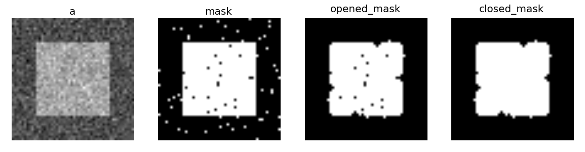
行使
检查重建正方形的面积小于最初正方形的面积。(如果关闭步骤在开始之前执行,则会发生相反情况)。
对于灰色图像,侵蚀(resp。膨胀)相当于用最小值(或最大值)替换像素。最大值)中心位于感兴趣像素上的结构元素覆盖的像素之间。
>>> a = np.zeros((7, 7), dtype=np.int)
>>> a[1:6, 1:6] = 3
>>> a[4, 4] = 2; a[2, 3] = 1
>>> a
array([[0, 0, 0, 0, 0, 0, 0],
       [0, 3, 3, 3, 3, 3, 0],
       [0, 3, 3, 1, 3, 3, 0],
       [0, 3, 3, 3, 3, 3, 0],
       [0, 3, 3, 3, 2, 3, 0],
       [0, 3, 3, 3, 3, 3, 0],
       [0, 0, 0, 0, 0, 0, 0]])
>>> ndimage.grey_erosion(a, size=(3, 3))
array([[0, 0, 0, 0, 0, 0, 0],
       [0, 0, 0, 0, 0, 0, 0],
       [0, 0, 1, 1, 1, 0, 0],
       [0, 0, 1, 1, 1, 0, 0],
       [0, 0, 3, 2, 2, 0, 0],
       [0, 0, 0, 0, 0, 0, 0],
       [0, 0, 0, 0, 0, 0, 0]])
1.5.10.4. 图像测量
让我们先生成一个很好的合成二进制图像。
>>> x, y = np.indices((100, 100))
>>> sig = np.sin(2*np.pi*x/50.) * np.sin(2*np.pi*y/50.) * (1+x*y/50.**2)**2
>>> mask = sig > 1
现在我们查看有关图像中对象的各种信息:
>>> labels, nb = ndimage.label(mask)
>>> nb
8
>>> areas = ndimage.sum(mask, labels, range(1, labels.max()+1))
>>> areas
array([ 190.,   45.,  424.,  278.,  459.,  190.,  549.,  424.])
>>> maxima = ndimage.maximum(sig, labels, range(1, labels.max()+1))
>>> maxima
array([  1.80238238,   1.13527605,   5.51954079,   2.49611818,
         6.71673619,   1.80238238,  16.76547217,   5.51954079])
>>> ndimage.find_objects(labels==4)
[(slice(30L, 48L, None), slice(30L, 48L, None))]
>>> sl = ndimage.find_objects(labels==4)
>>> import pylab as pl
>>> pl.imshow(sig[sl[0]])
<matplotlib.image.AxesImage object at ...>
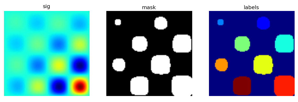
请参阅Image processing application: counting bubbles and unmolten grains以获得更高级的示例。
1.5.11. 科学计算总结练习 
总结练习主要使用Numpy,Scipy和Matplotlib。他们提供了一些Python实际科学计算的例子。现在已经介绍了使用Numpy和Scipy的基础知识,欢迎感兴趣的用户尝试这些练习。
锻炼: T0>
建议的解决方案: