入门¶

这些教程并不能成为研究生或本科生的机器学习课程，但我们可以快速概览一些重要的概念（和符号），以确保我们保持同一进度。你还需要下载本章中提到的数据集，以便运行后面教程中的示例代码。

下载¶

在每个学习算法页面上，你都可以下载相应的文件。如果你想同时下载所有的文件，你可以克隆教程的git仓库：

git clone https://github.com/lisa-lab/DeepLearningTutorials.git

数据集¶

MNIST数据集¶

(mnist.pkl.gz)

MNIST数据集由手写数字图像组成，它包括60,000个训练样本和10,000个测试样本。在许多论文以及本教程中，这60,000个训练样本被划分为50,000个实际训练样本集和10,000个交叉验证样本（用于选择超参数，如学习率和模型大小）。所有数字图像的数值大小已经过标准化处理，且每张图片的大小都为28×28像素。在原始数据集中，图像的每个像素由0和255之间的值表示，其中0是黑色，255是白色，中间的任何值是不同的灰度。

Here are some examples of MNIST digits:

为了方便起见，我们序列化(pickle)了数据集，以使其更容易在python中使用。It is available for download here. 这个序列化文件是一个由3个列表组成的元组，分别是：训练集、验证集和测试集。这三个列表中的每个列表都是由形如（图像列表，图像类别）组成的对。每个图像都用一个一维numpy数组表示，它含有784（28×28）个浮点值，每个值的取值范围在0~1之间（0表示黑色，1表示白色）。类别标签是0和9之间的数字，表示图像所代表的数字。The code block below shows how to load the dataset.
import cPickle, gzip, numpy

# Load the dataset
f = gzip.open('mnist.pkl.gz', 'rb')
train_set, valid_set, test_set = cPickle.load(f)
f.close()
当使用数据集时，我们通常将其分为minibatches（参见随机梯度下降）。我们推荐你将数据集存储到共享变量中，并在给定固定和已知批量（batch）大小的情况下基于minibatch索引访问它。使用共享变量的原因与使用GPU有关。将数据复制到GPU内存时会有很大的功耗。如果是根据代码运行的需要而复制数据（每个minibatch在需要时单独复制），因为上述消耗的存在，如果你不使用共享变量，GPU代码并不会比CPU代码（甚至更慢）快得多。然而如果你将数据保存在Theano的共享变量里，在构建共享变量时，Theano只需一次单独的调用即可复制GPU上的所有数据。之后，GPU可以通过从这个共享变量取一个切片来访问任何minibatch，而无需从CPU内存中复制任何信息，从而提高了效率。Because the datapoints and their labels are usually of different nature (labels are usually integers while datapoints are real numbers) we suggest to use different variables for label and data. 此外，我们建议对训练集、验证集和测试集使用不同的变量，以使代码更有可读性（结果有6个不同的共享变量）。

因为现在数据在一个变量中，并且一个minibatch被定义为该变量的一个切片，通过指明索引和大小来定义minibatch要更加自然。在我们的设置中，batch的大小在代码执行过程中保持不变，因此，一个函数实际上只需要索引来标识在哪个数据点工作。The code below shows how to store your data and how to access a minibatch:
def shared_dataset(data_xy):
    """ Function that loads the dataset into shared variables

    The reason we store our dataset in shared variables is to allow
    Theano to copy it into the GPU memory (when code is run on GPU).
    Since copying data into the GPU is slow, copying a minibatch everytime
    is needed (the default behaviour if the data is not in a shared
    variable) would lead to a large decrease in performance.
    """
    data_x, data_y = data_xy
    shared_x = theano.shared(numpy.asarray(data_x, dtype=theano.config.floatX))
    shared_y = theano.shared(numpy.asarray(data_y, dtype=theano.config.floatX))
    # When storing data on the GPU it has to be stored as floats
    # therefore we will store the labels as ``floatX`` as well
    # (``shared_y`` does exactly that). But during our computations
    # we need them as ints (we use labels as index, and if they are
    # floats it doesn't make sense) therefore instead of returning
    # ``shared_y`` we will have to cast it to int. This little hack
    # lets us get around this issue
    return shared_x, T.cast(shared_y, 'int32')

test_set_x, test_set_y = shared_dataset(test_set)
valid_set_x, valid_set_y = shared_dataset(valid_set)
train_set_x, train_set_y = shared_dataset(train_set)

batch_size = 500    # size of the minibatch

# accessing the third minibatch of the training set

data  = train_set_x[2 * batch_size: 3 * batch_size]
label = train_set_y[2 * batch_size: 3 * batch_size]

数据必须作为浮点数存储在GPU上（右侧的dtype表示在GPU上的存储类型，由theano.config.floatX给出）。为了解决标签的这个缺点，我们将它们存储为float，然后将其cast为int。

Note

如果你在GPU上运行代码，而且使用的数据集太大，不能容纳在内存中，代码就会崩溃。在这种情况下，你应该将数据存储在共享变量中。You can however store a sufficiently small chunk of your data (several minibatches) in a shared variable and use that during training. 一旦你使用完这个块，就更新它存储的值。这样你就可以最小化CPU内存和GPU内存之间的数据传输次数。

记号¶

数据集记号¶

We label data sets as $\mathcal{D}$ . 在需要加以区别时，我们将训练，验证和测试集合表示为： $\mathcal{D}_{train}$ ， $\mathcal{D}_{valid}$ 和 $\mathcal{D}_{test}$ 。The validation set is used to perform model selection and hyper-parameter selection, whereas the test set is used to evaluate the final generalization error and compare different algorithms in an unbiased way.

本教程主要处理分类问题，其中每个数据集 $\mathcal{D}$ 是由带索引的 $(x^{(i)},y^{(i)})$ 组成的数据集。我们使用上标来区分训练集样本：因此 $x^{(i)} \in \mathcal{R}^D$ 是第i个训练样本，它的维度为 $D$ 。类似地， $y^{(i)} \in \{0, ..., L\}$ 是输入 $x^{(i)}$ 对应的第i个标签。当 $y^{(i)}$ 具有其他类型时（例如，用于回归的高斯或用于预测多个符号的多项式组），可以很直接的将样本扩展到这种情况。

数学约定¶

$W$ ：大写的符号，表示一个矩阵，除非另有规定
$W_{ij}$ : element at i-th row and j-th column of matrix
$W_{i \cdot}, W_i$ ：向量，矩阵的第i行
$W_{\cdot j}$ ：向量，矩阵的第j列
$b$ ：小写的符号，表示一个向量，除非另有规定
$b_i$ : i-th element of vector

符号和首字母缩写列表¶

$D$ : number of input dimensions.
$D_h^{(i)}$ : number of hidden units in the $i$ -th layer.
$f_{\theta}(x)$ , $f(x)$ : classification function associated with a model $P(Y|x,\theta)$ , defined as ${\rm argmax}_k P(Y=k|x,\theta)$ . Note that we will often drop the $\theta$ subscript.
L: number of labels.
$\mathcal{L}(\theta, \cal{D})$ ：由参数 $\theta$ 定义的模型的对数似然函数 $\cal{D}$ 。
$\ell(\theta, \cal{D})$ ：参数为 $\theta$ 的预测函数f在数据集 $\cal{D}$ 上的经验损失。
NLL：负对数似然函数
$\theta$ : set of all parameters for a given model

Python命名空间¶

Tutorial code often uses the following namespaces:

import theano
import theano.tensor as T
import numpy

深度学习的监督优化的入门¶

深度学习最激动人心的是使用深层网络的无监督学习。But supervised learning also plays an important role. The utility of unsupervised pre-training is often evaluated on the basis of what performance can be achieved after supervised fine-tuning. 本章回顾分类模型的监督学习的基础知识，并且涵盖minibatch随机随机梯度下降算法，它用于微调本深度学习教程中的许多模型。请查看这些基于梯度学习的入门课程说明，了解有关使用梯度优化训练标准概念的更多基础知识。

学习一个分类器¶

0-1损失¶

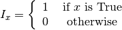
本深度学习教程中提供的模型主要用于分类。训练分类器的目的是最小化未见示例中的错误数量（0-1损失）。If $f: R^D \rightarrow \{0,...,L\}$ is the prediction function, then this loss can be written as:

$\ell_{0,1} = \sum_{i=0}^{|\mathcal{D}|} I_{f(x^{(i)}) \neq y^{(i)}}$

其中 $\mathcal{D}$ 是训练集合（在训练期间）或者也可以写为 $\mathcal{D} \cap \mathcal{D}_{train} = \emptyset$ （以避免使得评估验证集或测试集的错误具有偏向）。 $I$ 是试性函数，定义为：

$I_x = \left\{\begin{array}{ccc} 1&\mbox{ if $x$ is True} \\ 0&\mbox{ otherwise}\end{array}\right.$

In this tutorial, $f$ is defined as:

$f(x) = {\rm argmax}_k P(Y=k | x, \theta)$

In python, using Theano this can be written as :

# zero_one_loss is a Theano variable representing a symbolic
# expression of the zero one loss ; to get the actual value this
# symbolic expression has to be compiled into a Theano function (see
# the Theano tutorial for more details)
zero_one_loss = T.sum(T.neq(T.argmax(p_y_given_x), y))

负对数似然损失¶

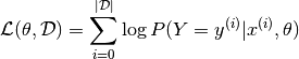
由于零一损失不可微分，因此对于大型模型（数千或数百万参数）进行优化代价很大（计算上的）。We thus maximize the log-likelihood of our classifier given all the labels in a training set.

$\mathcal{L}(\theta, \mathcal{D}) = \sum_{i=0}^{|\mathcal{D}|} \log P(Y=y^{(i)} | x^{(i)}, \theta)$

正确类的似然性与正确预测的数量不同，但是从随机初始化的分类器的角度来看，它们非常相似。记住，似然性和零一损失是不同的目标；你可以看到，它们在验证集中相关联，但有时一个会上升，而另一个下降，或反之亦然。

由于我们通常在讲使损失函数最小化，因此学习将尝试最小化负对数似然函数（NLL），定义为：

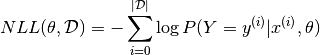
$NLL(\theta, \mathcal{D}) = - \sum_{i=0}^{|\mathcal{D}|} \log P(Y=y^{(i)} | x^{(i)}, \theta)$

分类器的NLL是0-1损失的可微分替代，我们使用该函数在训练数据上的梯度作为分类器深度学习的监督学习的讯号。

这可以使用以下代码进行计算：

# NLL is a symbolic variable ; to get the actual value of NLL, this symbolic
# expression has to be compiled into a Theano function (see the Theano
# tutorial for more details)
NLL = -T.sum(T.log(p_y_given_x)[T.arange(y.shape[0]), y])
# note on syntax: T.arange(y.shape[0]) is a vector of integers [0,1,2,...,len(y)].
# Indexing a matrix M by the two vectors [0,1,...,K], [a,b,...,k] returns the
# elements M[0,a], M[1,b], ..., M[K,k] as a vector.  Here, we use this
# syntax to retrieve the log-probability of the correct labels, y.

随机梯度下降¶

What is ordinary gradient descent? 它是一个简单的算法，在这个算法中我们在由包含一些参数的损失函数定义的误差曲面上，向下重复着进行小的步长。为了计算普通梯度下降，我们考虑让损失函数利用所有训练数据。Then the pseudocode of this algorithm can be described as :

# GRADIENT DESCENT

while True:
    loss = f(params)
    d_loss_wrt_params = ... # compute gradient
    params -= learning_rate * d_loss_wrt_params
    if <stopping condition is met>:
        return params

随机梯度下降（SGD）根据与普通梯度下降相同的原理工作，但一次只利用几个样本而不是整个训练集合来估计梯度，这样算法能更快地进行。在最简单的形式下，我们一次只利用一个单一的样本估计梯度。

# STOCHASTIC GRADIENT DESCENT
for (x_i,y_i) in training_set:
                            # imagine an infinite generator
                            # that may repeat examples (if there is only a finite training set)
    loss = f(params, x_i, y_i)
    d_loss_wrt_params = ... # compute gradient
    params -= learning_rate * d_loss_wrt_params
    if <stopping condition is met>:
        return params

我们所推荐的用于深度学习的变体，是使用所谓的“minibatches”的随机梯度下降法的一大转变。Minibatch SGD（MSGD）的工作原理与SGD相同，除了我们每次使用多个训练样本来估计梯度。这种技术减少了梯度估计中的方差，并且往往能更好地利用现代计算机中的分层存储器组织。

for (x_batch,y_batch) in train_batches:
                            # imagine an infinite generator
                            # that may repeat examples
    loss = f(params, x_batch, y_batch)
    d_loss_wrt_params = ... # compute gradient using theano
    params -= learning_rate * d_loss_wrt_params
    if <stopping condition is met>:
        return params

在选择minibatch大小 $B$ 时会有所权衡。The reduction of variance and use of SIMD instructions helps most when increasing $B$ from 1 to 2, but the marginal improvement fades rapidly to nothing. 对于大的 $B$ ，时间会被浪费在减少梯度估计的方差上，该时间还不如花在额外的梯度步骤上。最优的 $B$ 是与模型、数据集和硬件相关的，可以是从一到几百。在教程中我们将其设置为20，但这个几乎是一个任意的选择（虽然无害）。

Note

如果你训练固定数量的epoch，那么minibatch的大小将变得很重要，因为它控制了你的参数的更新次数。使用batch大小为1且训练10个epoch的模型产生的结果，与相同的10个epoch但是批次大小为20的训练相比产生完全不同的结果。当在不同batch大小之间切换时，请记住这一点，并且准备好根据所使用的batch大小来调整所有的其他参数。

上面的所有代码块展示了算法大概的伪代码。要在Theano中实现这样的算法可以按如下进行：

# Minibatch Stochastic Gradient Descent

# assume loss is a symbolic description of the loss function given
# the symbolic variables params (shared variable), x_batch, y_batch;

# compute gradient of loss with respect to params
d_loss_wrt_params = T.grad(loss, params)

# compile the MSGD step into a theano function
updates = [(params, params - learning_rate * d_loss_wrt_params)]
MSGD = theano.function([x_batch,y_batch], loss, updates=updates)

for (x_batch, y_batch) in train_batches:
    # here x_batch and y_batch are elements of train_batches and
    # therefore numpy arrays; function MSGD also updates the params
    print('Current loss is ', MSGD(x_batch, y_batch))
    if stopping_condition_is_met:
        return params

正则化¶

除了最优化，机器学习还有很多内容。当我们从数据训练我们的模型时，我们试图让它在新的样本中工作得很好，而不是它已经看到的示例。以上对于MSGD的训练循环没有考虑这一点，并且可能过度拟合训练样本。减少过度拟合的一种方法是使用正则化。正则化包括了好几种方法，而我们要在这里说明的是L1/L2正则化和提前停止。

L1和L2正则化¶

L1和L2正则化会向损失函数添加额外项，它会惩罚某些参数的配置。Formally, if our loss function is:

$NLL(\theta, \mathcal{D}) = - \sum_{i=0}^{|\mathcal{D}|} \log P(Y=y^{(i)} | x^{(i)}, \theta)$

那么正则化损失函数将是：

$E(\theta, \mathcal{D}) = NLL(\theta, \mathcal{D}) + \lambda R(\theta)\\$

或者，在我们的例子中

$E(\theta, \mathcal{D}) = NLL(\theta, \mathcal{D}) + \lambda||\theta||_p^p$

其中

$||\theta||_p = \left(\sum_{j=0}^{|\theta|}{|\theta_j|^p}\right)^{\frac{1}{p}}$

which is the $L_p$ norm of $\theta$ . $\lambda$ is a hyper-parameter which controls the relative importance of the regularization parameter. p的常用值为1和2，因此被称为L1/L2范数。如果p=2，则正则化矩阵也称为“权重衰减”。

原则上，对损失函数添加正则化项将促进神经网络中的平滑网络映射（通过惩罚大的参数值而实现，这减少了网络模型的非线性的量）。更直观地，两个项（NLL和 $R(\theta)$ ）对应于对数据很好地（NLL）建模并具有“朴素”或“平滑”解（ $R(\theta)$ ）。因此，最小化两者的和将理论上可以权衡训练数据的拟合与所发现的解的“一般性”。为了遵循奥卡姆剃刀(Occam's razor)原则，这个最小化过程应该能找到可以拟合训练数据的最简单的解（由我们的朴素准则度量）。

请注意，一个“朴素”的解并不意味着它具有很好的泛化性。根据实际经验，我们会发现在神经网络中实施正则化有助于泛化，特别是对小数据集来说。下面的代码块演示了如何用python计算同时包含权重系数分别为 $lambda_1$ 和 $lambda_2$ 的L1，L2正则化项的损失函数

# symbolic Theano variable that represents the L1 regularization term
L1  = T.sum(abs(param))

# symbolic Theano variable that represents the squared L2 term
L2 = T.sum(param ** 2)

# the loss
loss = NLL + lambda_1 * L1 + lambda_2 * L2

提前停止¶

提前停止通过在验证集上监控模型的性能来防止过度拟合。验证集是一组我们从未用于梯度下降，但也不属于测试集的样本集。验证样本被认为是未来测试样本的代表。We can use them during training because they are not part of the test set. 如果在模型在验证集上表现出的性能不再有很大的改善，或者甚至随着进一步优化而开始退化，那么算法就会停止继续优化。

选择何时停止还需要加以判断，其中也有好几种方法，但本教程将要利用的是一个基于几何增加patience的策略。

# early-stopping parameters
patience = 5000  # look as this many examples regardless
patience_increase = 2     # wait this much longer when a new best is
                              # found
improvement_threshold = 0.995  # a relative improvement of this much is
                               # considered significant
validation_frequency = min(n_train_batches, patience/2)
                              # go through this many
                              # minibatches before checking the network
                              # on the validation set; in this case we
                              # check every epoch

best_params = None
best_validation_loss = numpy.inf
test_score = 0.
start_time = time.clock()

done_looping = False
epoch = 0
while (epoch < n_epochs) and (not done_looping):
    # Report "1" for first epoch, "n_epochs" for last epoch
    epoch = epoch + 1
    for minibatch_index in range(n_train_batches):

        d_loss_wrt_params = ... # compute gradient
        params -= learning_rate * d_loss_wrt_params # gradient descent

        # iteration number. We want it to start at 0.
        iter = (epoch - 1) * n_train_batches + minibatch_index
        # note that if we do `iter % validation_frequency` it will be
        # true for iter = 0 which we do not want. We want it true for
        # iter = validation_frequency - 1.
        if (iter + 1) % validation_frequency == 0:

            this_validation_loss = ... # compute zero-one loss on validation set

            if this_validation_loss < best_validation_loss:

                # improve patience if loss improvement is good enough
                if this_validation_loss < best_validation_loss * improvement_threshold:

                    patience = max(patience, iter * patience_increase)
                best_params = copy.deepcopy(params)
                best_validation_loss = this_validation_loss

        if patience <= iter:
            done_looping = True
            break

# POSTCONDITION:
# best_params refers to the best out-of-sample parameters observed during the optimization

如果我们在耗尽patience之前用完训练数据的batch，那么我们只需回到训练集的开头并重复。

Note

The validation_frequency should always be smaller than the patience. 在用完patience之前，代码应该至少检查两次它是如何运行。这是我们使用公式validation_frequency = min( value, patience/2.)的原因。

Note

在决定是否增加patience时，可以通过进行统计量显著性检验而不是简单的比较来改进该算法。

测试¶

退出循环后，best_params变量表示验证集上性能最佳的模型。如果我们在另一个模型类（或者甚至是另一个随机初始化模型）上重复此过程，我们都应该使用相同的训练/验证/测试数据，来获得其他性能最佳的模型。如果我们要选择最好的模型类或最佳的初始化模型，我们比较的是每个模型的best_validation_loss。当我们最终选择了我们认为是最好的（在验证数据上）的模型时，我们再返回模型在测试集上的性能。这就是我们对未知示例的所期望的表现。

简要概括¶

That’s it for the optimization section. 提前停止的方法需要我们将样本集分成三组（训练集 $\mathcal{D}_{train}$ 、验证集 $\mathcal{D}_{valid}$ 、测试集 $\mathcal{D}_{test}$ ）。训练集被用于目标函数可微近似的minibatch随机梯度下降。当我们在实施梯度下降时，我们周期性地参考验证集，看看我们的模型是在真实（或至少是我们经验估计）的目标函数上表现如何。当我们在验证集上看到一个好的模型时，我们将它保存下来。当看到一个好的模型已经很久以来，我们放弃了我们的搜索并返回找到的最佳参数，以便在测试集上进行评估。

Theano/Python技巧¶

加载和保存模型¶

当你做实验时，它可能会需要好几个小时（有时需要好几天！），来为梯度下降找到最好的参数。一旦你找到它们，你会想要保存这些权重。你可能还想要在搜索继续进行的同时保存当前最佳估计值。

从共享变量中序列化numpy ndarrays

The best way to save/archive your model’s parameters is to use pickle or deepcopy the ndarray objects. 例如，如果你的参数在共享变量w, v, u中，那么你的保存命令应该像这样写：

>>> import cPickle
>>> save_file = open('path', 'wb')  # this will overwrite current contents
>>> cPickle.dump(w.get_value(borrow=True), save_file, -1)  # the -1 is for HIGHEST_PROTOCOL
>>> cPickle.dump(v.get_value(borrow=True), save_file, -1)  # .. and it triggers much more efficient
>>> cPickle.dump(u.get_value(borrow=True), save_file, -1)  # .. storage than numpy's default
>>> save_file.close()

Then later, you can load your data back like this:

>>> save_file = open('path')
>>> w.set_value(cPickle.load(save_file), borrow=True)
>>> v.set_value(cPickle.load(save_file), borrow=True)
>>> u.set_value(cPickle.load(save_file), borrow=True)

这种方法略微有些繁琐，但它屡试不爽。即便已经存储了多年，你依然可以加载数据，并在matplotlib中轻松地将它绘制出来。

不要为了长期存储而pickle你的训练函数或测试函数

Theano函数与Python的deepcopy和pickle原理兼容，但你没有必要pickle一个Theano函数。如果你更新了Theano文件夹和一个内部变化，那么你可能会无法反序列化（un-pickle）模型。Theano现在仍在不断的开发中，内部API可能会发生变化。因此，为了安全起见 - 不要为了长期存储而pickle整个训练或测试函数。pickle机制旨在用于短期存储，例如临时文件，或者在分布式作业中拷贝一个副本到另一台机器。

Read more about serialization in Theano, or Python’s pickling.

绘制中间结果¶

可视化可以是非常强大的工具，用于了解你的模型或训练算法正在做什么。你可能会试着在模型训练脚本中插入matplotlib绘图命令或PIL图像渲染命令。然而，后来你会在那些预渲染的图像中观察到一些有趣的东西，并想调查一下，但是从图片上看不是很清楚。You’ll wished you had saved the original model.

如果你有足够的磁盘空间，你的训练脚本应保存中间模型，可视化脚本应处理这些保存的模型。

你已经有了一个保存模型的函数不是吗？Just use it again to save these intermediate models.

你想知道的库：Python图像库（PIL）、matplotlib。

Table Of Contents

Previous topic

Next topic

This Page

入门¶

下载¶

数据集¶

MNIST数据集¶

记号¶

数据集记号¶

数学约定¶

符号和首字母缩写列表¶

Python命名空间¶

深度学习的监督优化的入门¶

学习一个分类器¶

0-1损失¶

负对数似然损失¶

随机梯度下降¶

正则化¶

L1和L2正则化¶

提前停止¶

测试¶

简要概括¶

Theano/Python技巧¶

加载和保存模型¶

绘制中间结果¶