Hybrid Monte-Carlo Sampling¶

Note

This is an advanced tutorial, which shows how one can implemented Hybrid Monte-Carlo (HMC) sampling using Theano. We assume the reader is already familiar with Theano and energy-based models such as the RBM.

Note

The code for this section is available for download here.

理论¶

Maximum likelihood learning of energy-based models requires a robust algorithm to sample negative phase particles (see Eq. (4) of the Restricted Boltzmann Machines (RBM) tutorial). When training RBMs with CD or PCD, this is typically done with block Gibbs sampling, where the conditional distributions $p(h|v)$ and $p(v|h)$ are used as the transition operators of the Markov chain.

In certain cases however, these conditional distributions might be difficult to sample from (i.e. requiring expensive matrix inversions, as in the case of the “mean-covariance RBM”). Also, even if Gibbs sampling can be done efficiently, it nevertheless operates via a random walk which might not be statistically efficient for some distributions. In this context, and when sampling from continuous variables, Hybrid Monte Carlo (HMC) can prove to be a powerful tool [Duane87]. It avoids random walk behavior by simulating a physical system governed by Hamiltonian dynamics, potentially avoiding tricky conditional distributions in the process.

In HMC, model samples are obtained by simulating a physical system, where particles move about a high-dimensional landscape, subject to potential and kinetic energies. Adapting the notation from [Neal93], particles are characterized by a position vector or state $s \in \mathcal{R}^D$ and velocity vector $\phi \in \mathcal{R}^D$ . The combined state of a particle is denoted as $\chi=(s,\phi)$ . The Hamiltonian is then defined as the sum of potential energy $E(s)$ (same energy function defined by energy-based models) and kinetic energy $K(\phi)$ , as follows:

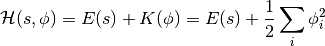
$\mathcal{H}(s,\phi) = E(s) + K(\phi) = E(s) + \frac{1}{2} \sum_i \phi_i^2$

Instead of sampling $p(s)$ directly, HMC operates by sampling from the canonical distribution $p(s,\phi) = \frac{1}{Z} \exp(-\mathcal{H}(s,\phi))=p(s)p(\phi)$ . Because the two variables are independent, marginalizing over $\phi$ is trivial and recovers the original distribution of interest.

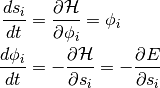
Hamiltonian Dynamics

State $s$ and velocity $\phi$ are modified such that $\mathcal{H}(s,\phi)$ remains constant throughout the simulation. The differential equations are given by:

(1) $\frac{ds_i}{dt} &= \frac{\partial \mathcal{H}}{\partial \phi_i} = \phi_i \\ \frac{d\phi_i}{dt} &= - \frac{\partial \mathcal{H}}{\partial s_i} = - \frac{\partial E}{\partial s_i}$

As shown in [Neal93], the above transformation preserves volume and is reversible. The above dynamics can thus be used as transition operators of a Markov chain and will leave $p(s,\phi)$ invariant. That chain by itself is not ergodic however, since simulating the dynamics maintains a fixed Hamiltonian $\mathcal{H}(s,\phi)$ . HMC thus alternates hamiltonian dynamic steps, with Gibbs sampling of the velocity. Because $p(s)$ and $p(\phi)$ are independent, sampling 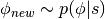$\phi_{new} \sim p(\phi|s)$ is trivial since 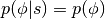$p(\phi|s)=p(\phi)$ , where $p(\phi)$ is often taken to be the uni-variate Gaussian.

The Leap-Frog Algorithm

In practice, we cannot simulate Hamiltonian dynamics exactly because of the problem of time discretization. There are several ways one can do this. To maintain invariance of the Markov chain however, care must be taken to preserve the properties of volume conservation and time reversibility. The leap-frog algorithm maintains these properties and operates in 3 steps:

(2) $\phi_i(t + \epsilon/2) &= \phi_i(t) - \frac{\epsilon}{2} \frac{\partial{}}{\partial s_i} E(s(t)) \\ s_i(t + \epsilon) &= s_i(t) + \epsilon \phi_i(t + \epsilon/2) \\ \phi_i(t + \epsilon) &= \phi_i(t + \epsilon/2) - \frac{\epsilon}{2} \frac{\partial{}}{\partial s_i} E(s(t + \epsilon)) \\$

We thus perform a half-step update of the velocity at time $t+\epsilon/2$ , which is then used to compute $s(t + \epsilon)$ and $\phi(t + \epsilon)$ .

Accept / Reject

In practice, using finite stepsizes $\epsilon$ will not preserve $\mathcal{H}(s,\phi)$ exactly and will introduce bias in the simulation. Also, rounding errors due to the use of floating point numbers means that the above transformation will not be perfectly reversible.

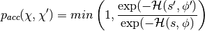
HMC cancels these effects exactly by adding a Metropolis accept/reject stage, after $n$ leapfrog steps. The new state $\chi' = (s',\phi')$ is accepted with probability $p_{acc}(\chi,\chi')$ , defined as:

$p_{acc}(\chi,\chi') = min \left( 1, \frac{\exp(-\mathcal{H}(s',\phi')}{\exp(-\mathcal{H}(s,\phi)} \right)$

HMC Algorithm

In this tutorial, we obtain a new HMC sample as follows:

sample a new velocity from a univariate Gaussian distribution
perform $n$ leapfrog steps to obtain the new state
perform accept/reject move of

使用Theano实现HMC¶

In Theano, update dictionaries and shared variables provide a natural way to implement a sampling algorithm. The current state of the sampler can be represented as a Theano shared variable, with HMC updates being implemented by the updates list of a Theano function.

We breakdown the HMC algorithm into the following sub-components:

$simulate\_dynamics$ : a symbolic Python function which, given an initial position and velocity, will perform $n\_steps$ leapfrog updates and return the symbolic variables for the proposed state $\chi'$ .
$hmc\_move$ : a symbolic Python function which given a starting position, generates $\chi$ by randomly sampling a velocity vector. It then calls $simulate\_dynamics$ and determines whether the transition $\chi \rightarrow \chi'$ is to be accepted.
$hmc\_updates$ : a Python function which, given the symbolic outputs of $hmc\_move$ , generates the list of updates for a single iteration of HMC.
$HMC\_sampler$ : a Python helper class which wraps everything together.

simulate_dynamics

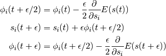
To perform $n$ leapfrog steps, we first need to define a function over which $Scan$ can iterate over. Instead of implementing Eq. (2) verbatim, notice that we can obtain $s(t + n \epsilon)$ and $\phi(t + n \epsilon)$ by performing an initial half-step update for $\phi$ , followed by $n$ full-step updates for $s,\phi$ and one last half-step update for $\phi$ . In loop form, this gives:

(3) $& \phi_i(t + \epsilon/2) = \phi_i(t) - \frac{\epsilon}{2} \frac{\partial{}}{\partial s_i} E(s(t)) \\ & s_i(t + \epsilon) = s_i(t) + \epsilon \phi_i(t + \epsilon/2) \\ & \text{For } m \in [2,n]\text{, perform full updates: } \\ & \qquad \phi_i(t + (m - 1/2)\epsilon) = \phi_i(t + (m-3/2)\epsilon) - \epsilon \frac{\partial{}}{\partial s_i} E(s(t + (m-1)\epsilon)) \\ & \qquad s_i(t + m\epsilon) = s_i(t) + \epsilon \phi_i(t + (m-1/2)\epsilon) \\ & \phi_i(t + n\epsilon) = \phi_i(t + (n-1/2)\epsilon) - \frac{\epsilon}{2} \frac{\partial{}}{\partial s_i} E(s(t + n\epsilon)) \\$

The inner-loop defined above is implemented by the following $leapfrog$ function, with $pos$ , $vel$ and $step$ replacing $s,\phi$ and $\epsilon$ respectively.

    def leapfrog(pos, vel, step):
        """
        Inside loop of Scan. Performs one step of leapfrog update, using
        Hamiltonian dynamics.

        Parameters
        ----------
        pos: theano matrix
            in leapfrog update equations, represents pos(t), position at time t
        vel: theano matrix
            in leapfrog update equations, represents vel(t - stepsize/2),
            velocity at time (t - stepsize/2)
        step: theano scalar
            scalar value controlling amount by which to move

        Returns
        -------
        rval1: [theano matrix, theano matrix]
            Symbolic theano matrices for new position pos(t + stepsize), and
            velocity vel(t + stepsize/2)
        rval2: dictionary
            Dictionary of updates for the Scan Op
        """
        # from pos(t) and vel(t-stepsize//2), compute vel(t+stepsize//2)
        dE_dpos = TT.grad(energy_fn(pos).sum(), pos)
        new_vel = vel - step * dE_dpos
        # from vel(t+stepsize//2) compute pos(t+stepsize)
        new_pos = pos + step * new_vel
        return [new_pos, new_vel], {}

The $simulate\_dynamics$ function performs the full algorithm of Eqs. (3). We start with the initial half-step update of $\phi$ and full-step of $s$ , and then scan over the $leapfrog$ method $n\_steps-1$ times.

def simulate_dynamics(initial_pos, initial_vel, stepsize, n_steps, energy_fn):
    """
    Return final (position, velocity) obtained after an `n_steps` leapfrog
    updates, using Hamiltonian dynamics.

    Parameters
    ----------
    initial_pos: shared theano matrix
        Initial position at which to start the simulation
    initial_vel: shared theano matrix
        Initial velocity of particles
    stepsize: shared theano scalar
        Scalar value controlling amount by which to move
    energy_fn: python function
        Python function, operating on symbolic theano variables, used to
        compute the potential energy at a given position.

    Returns
    -------
    rval1: theano matrix
        Final positions obtained after simulation
    rval2: theano matrix
        Final velocity obtained after simulation
    """

    def leapfrog(pos, vel, step):
        """
        Inside loop of Scan. Performs one step of leapfrog update, using
        Hamiltonian dynamics.

        Parameters
        ----------
        pos: theano matrix
            in leapfrog update equations, represents pos(t), position at time t
        vel: theano matrix
            in leapfrog update equations, represents vel(t - stepsize/2),
            velocity at time (t - stepsize/2)
        step: theano scalar
            scalar value controlling amount by which to move

        Returns
        -------
        rval1: [theano matrix, theano matrix]
            Symbolic theano matrices for new position pos(t + stepsize), and
            velocity vel(t + stepsize/2)
        rval2: dictionary
            Dictionary of updates for the Scan Op
        """
        # from pos(t) and vel(t-stepsize//2), compute vel(t+stepsize//2)
        dE_dpos = TT.grad(energy_fn(pos).sum(), pos)
        new_vel = vel - step * dE_dpos
        # from vel(t+stepsize//2) compute pos(t+stepsize)
        new_pos = pos + step * new_vel
        return [new_pos, new_vel], {}

    # compute velocity at time-step: t + stepsize//2
    initial_energy = energy_fn(initial_pos)
    dE_dpos = TT.grad(initial_energy.sum(), initial_pos)
    vel_half_step = initial_vel - 0.5 * stepsize * dE_dpos

    # compute position at time-step: t + stepsize
    pos_full_step = initial_pos + stepsize * vel_half_step

    # perform leapfrog updates: the scan op is used to repeatedly compute
    # vel(t + (m-1/2)*stepsize) and pos(t + m*stepsize) for m in [2,n_steps].
    (all_pos, all_vel), scan_updates = theano.scan(
        leapfrog,
        outputs_info=[
            dict(initial=pos_full_step),
            dict(initial=vel_half_step),
        ],
        non_sequences=[stepsize],
        n_steps=n_steps - 1)
    final_pos = all_pos[-1]
    final_vel = all_vel[-1]
    # NOTE: Scan always returns an updates dictionary, in case the
    # scanned function draws samples from a RandomStream. These
    # updates must then be used when compiling the Theano function, to
    # avoid drawing the same random numbers each time the function is
    # called. In this case however, we consciously ignore
    # "scan_updates" because we know it is empty.
    assert not scan_updates

    # The last velocity returned by scan is vel(t +
    # (n_steps - 1 / 2) * stepsize) We therefore perform one more half-step
    # to return vel(t + n_steps * stepsize)
    energy = energy_fn(final_pos)
    final_vel = final_vel - 0.5 * stepsize * TT.grad(energy.sum(), final_pos)

    # return new proposal state
    return final_pos, final_vel

A final half-step is performed to compute $\phi(t+n\epsilon)$ , and the final proposed state $\chi'$ is returned.

hmc_move

The $hmc\_move$ function implements the remaining steps (steps 1 and 3) of an HMC move proposal (while wrapping the $simulate\_dynamics$ function). Given a matrix of initial states $s \in \mathcal{R}^{N \times D}$ ( $positions$ ) and energy function $E(s)$ ( $energy\_fn$ ), it defines the symbolic graph for computing $n\_steps$ of HMC, using a given $stepsize$ . The function prototype is as follows:

def hmc_move(s_rng, positions, energy_fn, stepsize, n_steps):
    """
    This function performs one-step of Hybrid Monte-Carlo sampling. We start by
    sampling a random velocity from a univariate Gaussian distribution, perform
    `n_steps` leap-frog updates using Hamiltonian dynamics and accept-reject
    using Metropolis-Hastings.

    Parameters
    ----------
    s_rng: theano shared random stream
        Symbolic random number generator used to draw random velocity and
        perform accept-reject move.
    positions: shared theano matrix
        Symbolic matrix whose rows are position vectors.
    energy_fn: python function
        Python function, operating on symbolic theano variables, used to
        compute the potential energy at a given position.
    stepsize:  shared theano scalar
        Shared variable containing the stepsize to use for `n_steps` of HMC
        simulation steps.
    n_steps: integer
        Number of HMC steps to perform before proposing a new position.

    Returns
    -------
    rval1: boolean
        True if move is accepted, False otherwise
    rval2: theano matrix
        Matrix whose rows contain the proposed "new position"
    """

We start by sampling random velocities, using the provided shared RandomStream object. Velocities are sampled independently for each dimension and for each particle under simulation, yielding a $N \times D$ matrix.

    # sample random velocity
    initial_vel = s_rng.normal(size=positions.shape)

Since we now have an initial position and velocity, we can now call the $simulate\_dynamics$ to obtain the proposal for the new state $\chi'$ .

    # perform simulation of particles subject to Hamiltonian dynamics
    final_pos, final_vel = simulate_dynamics(
        initial_pos=positions,
        initial_vel=initial_vel,
        stepsize=stepsize,
        n_steps=n_steps,
        energy_fn=energy_fn
    )

We then accept/reject the proposed state based on the Metropolis algorithm.

    # accept/reject the proposed move based on the joint distribution
    accept = metropolis_hastings_accept(
        energy_prev=hamiltonian(positions, initial_vel, energy_fn),
        energy_next=hamiltonian(final_pos, final_vel, energy_fn),
        s_rng=s_rng
    )

where $metropolis\_hastings\_accept$ and $hamiltonian$ are helper functions, defined as follows.

def metropolis_hastings_accept(energy_prev, energy_next, s_rng):
    """
    Performs a Metropolis-Hastings accept-reject move.

    Parameters
    ----------
    energy_prev: theano vector
        Symbolic theano tensor which contains the energy associated with the
        configuration at time-step t.
    energy_next: theano vector
        Symbolic theano tensor which contains the energy associated with the
        proposed configuration at time-step t+1.
    s_rng: theano.tensor.shared_randomstreams.RandomStreams
        Theano shared random stream object used to generate the random number
        used in proposal.

    Returns
    -------
    return: boolean
        True if move is accepted, False otherwise
    """
    ediff = energy_prev - energy_next
    return (TT.exp(ediff) - s_rng.uniform(size=energy_prev.shape)) >= 0

def hamiltonian(pos, vel, energy_fn):
    """
    Returns the Hamiltonian (sum of potential and kinetic energy) for the given
    velocity and position.

    Parameters
    ----------
    pos: theano matrix
        Symbolic matrix whose rows are position vectors.
    vel: theano matrix
        Symbolic matrix whose rows are velocity vectors.
    energy_fn: python function
        Python function, operating on symbolic theano variables, used tox
        compute the potential energy at a given position.

    Returns
    -------
    return: theano vector
        Vector whose i-th entry is the Hamiltonian at position pos[i] and
        velocity vel[i].
    """
    # assuming mass is 1
    return energy_fn(pos) + kinetic_energy(vel)

def kinetic_energy(vel):
    """Returns the kinetic energy associated with the given velocity
    and mass of 1.

    Parameters
    ----------
    vel: theano matrix
        Symbolic matrix whose rows are velocity vectors.

    Returns
    -------
    return: theano vector
        Vector whose i-th entry is the kinetic entry associated with vel[i].

    """
    return 0.5 * (vel ** 2).sum(axis=1)

$hmc\_move$ finally returns the tuple $(accept, final\_pos)$ . $accept$ is a symbolic boolean variable indicating whether or not the new state $final\_pos$ should be used or not.

hmc_updates

The purpose of $hmc\_updates$ is to generate the list of updates to perform, whenever our HMC sampling function is called. $hmc\_updates$ thus receives as parameters, a series of shared variables to update ( $positions$ , $stepsize$ and $avg\_acceptance\_rate$ ), and the parameters required to compute their new state.

def hmc_updates(positions, stepsize, avg_acceptance_rate, final_pos, accept,
                target_acceptance_rate, stepsize_inc, stepsize_dec,
                stepsize_min, stepsize_max, avg_acceptance_slowness):
    """This function is executed after `n_steps` of HMC sampling
    (`hmc_move` function). It creates the updates dictionary used by
    the `simulate` function. It takes care of updating: the position
    (if the move is accepted), the stepsize (to track a given target
    acceptance rate) and the average acceptance rate (computed as a
    moving average).

    Parameters
    ----------
    positions: shared variable, theano matrix
        Shared theano matrix whose rows contain the old position
    stepsize: shared variable, theano scalar
        Shared theano scalar containing current step size
    avg_acceptance_rate: shared variable, theano scalar
        Shared theano scalar containing the current average acceptance rate
    final_pos: shared variable, theano matrix
        Shared theano matrix whose rows contain the new position
    accept: theano scalar
        Boolean-type variable representing whether or not the proposed HMC move
        should be accepted or not.
    target_acceptance_rate: float
        The stepsize is modified in order to track this target acceptance rate.
    stepsize_inc: float
        Amount by which to increment stepsize when acceptance rate is too high.
    stepsize_dec: float
        Amount by which to decrement stepsize when acceptance rate is too low.
    stepsize_min: float
        Lower-bound on `stepsize`.
    stepsize_min: float
        Upper-bound on `stepsize`.
    avg_acceptance_slowness: float
        Average acceptance rate is computed as an exponential moving average.
        (1-avg_acceptance_slowness) is the weight given to the newest
        observation.

    Returns
    -------
    rval1: dictionary-like
        A dictionary of updates to be used by the `HMC_Sampler.simulate`
        function.  The updates target the position, stepsize and average
        acceptance rate.

    """

    # POSITION UPDATES #
    # broadcast `accept` scalar to tensor with the same dimensions as
    # final_pos.
    accept_matrix = accept.dimshuffle(0, *(('x',) * (final_pos.ndim - 1)))
    # if accept is True, update to `final_pos` else stay put
    new_positions = TT.switch(accept_matrix, final_pos, positions)

Using the above code, the dictionary ${positions: new\_positions}$ can be used to update the state of the sampler with either (1) the new state $final\_pos$ if $accept$ is True, or (2) the old state if $accept$ is False. This conditional assignment is performed by the switch op.

$switch$ expects as its first argument, a boolean mask with the same broadcastable dimensions as the second and third argument. Since $accept$ is scalar-valued, we must first use dimshuffle to transform it to a tensor with $final\_pos.ndim$ broadcastable dimensions ( $accept\_matrix$ ).

$hmc\_updates$ additionally implements an adaptive version of HMC, as implemented in the accompanying code to [Ranzato10]. We start by tracking the average acceptance rate of the HMC move proposals (across many simulations), using an exponential moving average with time constant $1-avg\_acceptance\_slowness$ .

    # ACCEPT RATE UPDATES #
    # perform exponential moving average
    mean_dtype = theano.scalar.upcast(accept.dtype, avg_acceptance_rate.dtype)
    new_acceptance_rate = TT.add(
        avg_acceptance_slowness * avg_acceptance_rate,
        (1.0 - avg_acceptance_slowness) * accept.mean(dtype=mean_dtype))

If the average acceptance rate is larger than the $target\_acceptance\_rate$ , we increase the $stepsize$ by a factor of $stepsize\_inc$ in order to increase the mixing rate of our chain. If the average acceptance rate is too low however, $stepsize$ is decreased by a factor of $stepsize\_dec$ , yielding a more conservative mixing rate. The clip op allows us to maintain the $stepsize$ in the range [ $stepsize\_min$ , $stepsize\_max$ ].

    # STEPSIZE UPDATES #
    # if acceptance rate is too low, our sampler is too "noisy" and we reduce
    # the stepsize. If it is too high, our sampler is too conservative, we can
    # get away with a larger stepsize (resulting in better mixing).
    _new_stepsize = TT.switch(avg_acceptance_rate > target_acceptance_rate,
                              stepsize * stepsize_inc, stepsize * stepsize_dec)
    # maintain stepsize in [stepsize_min, stepsize_max]
    new_stepsize = TT.clip(_new_stepsize, stepsize_min, stepsize_max)

The final updates list is then returned.

    return [(positions, new_positions),
            (stepsize, new_stepsize),
            (avg_acceptance_rate, new_acceptance_rate)]

HMC_sampler

We finally tie everything together using the $HMC\_Sampler$ class. Its main elements are:

$new\_from\_shared\_positions$ : a constructor method which allocates various shared variables and strings together the calls to $hmc\_move$ and $hmc\_updates$ . It also builds the theano function $simulate$ , whose sole purpose is to execute the updates generated by $hmc\_updates$ .
$draw$ : a convenience method which calls the Theano function $simulate$ and returns a copy of the contents of the shared variable $self.positions$ .

class HMC_sampler(object):
    """
    Convenience wrapper for performing Hybrid Monte Carlo (HMC). It creates the
    symbolic graph for performing an HMC simulation (using `hmc_move` and
    `hmc_updates`). The graph is then compiled into the `simulate` function, a
    theano function which runs the simulation and updates the required shared
    variables.

    Users should interface with the sampler thorugh the `draw` function which
    advances the markov chain and returns the current sample by calling
    `simulate` and `get_position` in sequence.

    The hyper-parameters are the same as those used by Marc'Aurelio's
    'train_mcRBM.py' file (available on his personal home page).
    """

    def __init__(self, **kwargs):
        self.__dict__.update(kwargs)

    @classmethod
    def new_from_shared_positions(
        cls,
        shared_positions,
        energy_fn,
        initial_stepsize=0.01,
        target_acceptance_rate=.9,
        n_steps=20,
        stepsize_dec=0.98,
        stepsize_min=0.001,
        stepsize_max=0.25,
        stepsize_inc=1.02,
        # used in geometric avg. 1.0 would be not moving at all
        avg_acceptance_slowness=0.9,
        seed=12345
    ):
        """
        :param shared_positions: theano ndarray shared var with
            many particle [initial] positions

        :param energy_fn:
            callable such that energy_fn(positions)
            returns theano vector of energies.
            The len of this vector is the batchsize.

            The sum of this energy vector must be differentiable (with
            theano.tensor.grad) with respect to the positions for HMC
            sampling to work.

        """
        # allocate shared variables
        stepsize = sharedX(initial_stepsize, 'hmc_stepsize')
        avg_acceptance_rate = sharedX(target_acceptance_rate,
                                      'avg_acceptance_rate')
        s_rng = theano.sandbox.rng_mrg.MRG_RandomStreams(seed)

        # define graph for an `n_steps` HMC simulation
        accept, final_pos = hmc_move(
            s_rng,
            shared_positions,
            energy_fn,
            stepsize,
            n_steps)

        # define the dictionary of updates, to apply on every `simulate` call
        simulate_updates = hmc_updates(
            shared_positions,
            stepsize,
            avg_acceptance_rate,
            final_pos=final_pos,
            accept=accept,
            stepsize_min=stepsize_min,
            stepsize_max=stepsize_max,
            stepsize_inc=stepsize_inc,
            stepsize_dec=stepsize_dec,
            target_acceptance_rate=target_acceptance_rate,
            avg_acceptance_slowness=avg_acceptance_slowness)

        # compile theano function
        simulate = function([], [], updates=simulate_updates)

        # create HMC_sampler object with the following attributes ...
        return cls(
            positions=shared_positions,
            stepsize=stepsize,
            stepsize_min=stepsize_min,
            stepsize_max=stepsize_max,
            avg_acceptance_rate=avg_acceptance_rate,
            target_acceptance_rate=target_acceptance_rate,
            s_rng=s_rng,
            _updates=simulate_updates,
            simulate=simulate)

    def draw(self, **kwargs):
        """
        Returns a new position obtained after `n_steps` of HMC simulation.

        Parameters
        ----------
        kwargs: dictionary
            The `kwargs` dictionary is passed to the shared variable
            (self.positions) `get_value()` function.  For example, to avoid
            copying the shared variable value, consider passing `borrow=True`.

        Returns
        -------
        rval: numpy matrix
            Numpy matrix whose of dimensions similar to `initial_position`.
       """
        self.simulate()
        return self.positions.get_value(borrow=False)

测试我们的采样器¶

We test our implementation of HMC by sampling from a multi-variate Gaussian distribution. We start by generating a random mean vector $mu$ and covariance matrix $cov$ , which allows us to define the energy function of the corresponding Gaussian distribution: $gaussian\_energy$ . We then initialize the state of the sampler by allocating a $position$ shared variable. It is passed to the constructor of $HMC\_sampler$ along with our target energy function.

Following a burn-in period, we then generate a large number of samples and compare the empirical mean and covariance matrix to their true values.

def sampler_on_nd_gaussian(sampler_cls, burnin, n_samples, dim=10):
    batchsize = 3

    rng = numpy.random.RandomState(123)

    # Define a covariance and mu for a gaussian
    mu = numpy.array(rng.rand(dim) * 10, dtype=theano.config.floatX)
    cov = numpy.array(rng.rand(dim, dim), dtype=theano.config.floatX)
    cov = (cov + cov.T) / 2.
    cov[numpy.arange(dim), numpy.arange(dim)] = 1.0
    cov_inv = numpy.linalg.inv(cov)

    # Define energy function for a multi-variate Gaussian
    def gaussian_energy(x):
        return 0.5 * (theano.tensor.dot((x - mu), cov_inv) *
                      (x - mu)).sum(axis=1)

    # Declared shared random variable for positions
    position = rng.randn(batchsize, dim).astype(theano.config.floatX)
    position = theano.shared(position)

    # Create HMC sampler
    sampler = sampler_cls(position, gaussian_energy,
                          initial_stepsize=1e-3, stepsize_max=0.5)

    # Start with a burn-in process
    garbage = [sampler.draw() for r in range(burnin)]  # burn-in Draw
    # `n_samples`: result is a 3D tensor of dim [n_samples, batchsize,
    # dim]
    _samples = numpy.asarray([sampler.draw() for r in range(n_samples)])
    # Flatten to [n_samples * batchsize, dim]
    samples = _samples.T.reshape(dim, -1).T

    print('****** TARGET VALUES ******')
    print('target mean:', mu)
    print('target cov:\n', cov)

    print('****** EMPIRICAL MEAN/COV USING HMC ******')
    print('empirical mean: ', samples.mean(axis=0))
    print('empirical_cov:\n', numpy.cov(samples.T))

    print('****** HMC INTERNALS ******')
    print('final stepsize', sampler.stepsize.get_value())
    print('final acceptance_rate', sampler.avg_acceptance_rate.get_value())

    return sampler

def test_hmc():
    sampler = sampler_on_nd_gaussian(HMC_sampler.new_from_shared_positions,
                                     burnin=1000, n_samples=1000, dim=5)
    assert abs(sampler.avg_acceptance_rate.get_value() -
               sampler.target_acceptance_rate) < .1
    assert sampler.stepsize.get_value() >= sampler.stepsize_min
    assert sampler.stepsize.get_value() <= sampler.stepsize_max

The above code can be run using the command: “nosetests -s code/hmc/test_hmc.py”. The output is as follows:

[desjagui@atchoum hmc]$ python test_hmc.py

****** TARGET VALUES ******
target mean: [ 6.96469186  2.86139335  2.26851454  5.51314769  7.1946897 ]
target cov:
[[ 1.          0.66197111  0.71141257  0.55766643  0.35753822]
 [ 0.66197111  1.          0.31053199  0.45455485  0.37991646]
 [ 0.71141257  0.31053199  1.          0.62800335  0.38004541]
 [ 0.55766643  0.45455485  0.62800335  1.          0.50807871]
 [ 0.35753822  0.37991646  0.38004541  0.50807871  1.        ]]

****** EMPIRICAL MEAN/COV USING HMC ******
empirical mean:  [ 6.94155164  2.81526039  2.26301715  5.46536853  7.19414496]
empirical_cov:
[[ 1.05152997  0.68393537  0.76038645  0.59930252  0.37478746]
 [ 0.68393537  0.97708159  0.37351422  0.48362404  0.3839558 ]
 [ 0.76038645  0.37351422  1.03797111  0.67342957  0.41529132]
 [ 0.59930252  0.48362404  0.67342957  1.02865056  0.53613649]
 [ 0.37478746  0.3839558   0.41529132  0.53613649  0.98721449]]

****** HMC INTERNALS ******
final stepsize 0.460446628091
final acceptance_rate 0.922502043428

As can be seen above, the samples generated by our HMC sampler yield an empirical mean and covariance matrix, which are very close to the true underlying parameters. The adaptive algorithm also seemed to work well as the final acceptance rate is close to our target of $0.9$ .

参考¶

[Alder59]

Alder, B. J. and Wainwright, T. E. (1959) “Studies in molecular dynamics.1. General method”, Journal of Chemical Physics, vol.31, pp.459-466.

[Andersen80]

Andersen, H.C. (1980) “Molecular dynamics simulations at constant pressure and/or temperature”, Journal of Chemical Physics, vol.72, pp.2384-2393.

[Duane87]

Duane, S., Kennedy, A. D., Pendleton, B. J., and Roweth, D. (1987) “Hybrid Monte Carlo”, Physics Letters, vol.195, pp.216-222.

[Neal93]

(1, 2) Neal, R. M. (1993) “Probabilistic Inference Using Markov Chain Monte Carlo Methods”, Technical Report CRG-TR-93-1, Dept.of Computer Science, University of Toronto, 144 pages

Table Of Contents

Previous topic

Next topic

This Page

Hybrid Monte-Carlo Sampling¶

理论¶

使用Theano实现HMC¶

测试我们的采样器¶

参考¶