注意
here下载完整的示例代码
计算机视觉迁移学习
在本教程中,你将学习如何使用迁移学习训练用于图像分类的卷积神经网络。 你可以在 cs231n 笔记 中阅读更多关于迁移学习的内容。
引用这些笔记,
实际上,很少有人从头开始训练整个卷积网络(随机初始化),因为拥有足够大小的数据集相对较少。 相反,通常要在非常大的数据集(例如 ImageNet)上预训练 ConvNet,该数据集包含 1000 个类别的 120 万个图像,然后将 ConvNet 用作初始化或固定要素提取器,用于感兴趣的任务。
这两个主要的转移学习方案如下所示:
微调 convnet:我们使用预先训练的网络(如在 Imagenet 1000 数据集上训练的网络)来初始化网络,而不是随机初始化。 其余的训练看起来和往常一样。
ConvNet 作为固定要素提取器:在这里,我们将冻结除最终完全连接层以外的所有网络的权重。 最后一个完全连接的图层将替换为具有随机权重的新图层,并且仅训练此图层。
# License: BSD
# Author: Sasank Chilamkurthy

from __future__ import print_function, division

import torch
import torch.nn as nn
import torch.optim as optim
from torch.optim import lr_scheduler
import numpy as np
import torchvision
from torchvision import datasets, models, transforms
import matplotlib.pyplot as plt
import time
import os
import copy

plt.ion()   # interactive mode
加载数据|
我们将使用 torchvision 和 torch.utils.data 包来加载数据。
我们今天要解决的问题是训练一个模型来分类蚂蚁和蜜蜂。 我们大约有120张蚂蚁和蜜蜂的训练图像。 每个类有 75 个验证映像。 通常,如果从头开始训练的话,这是一个非常小的数据集。 由于我们正在使用迁移学习,因此我们应该能够很好地泛化。
该数据集是 imagenet 的很小一部分。
注意
从此处下载数据并将其提取到当前目录。
# Data augmentation and normalization for training
# Just normalization for validation
data_transforms = {
    'train': transforms.Compose([
        transforms.RandomResizedCrop(224),
        transforms.RandomHorizontalFlip(),
        transforms.ToTensor(),
        transforms.Normalize([0.485, 0.456, 0.406], [0.229, 0.224, 0.225])
    ]),
    'val': transforms.Compose([
        transforms.Resize(256),
        transforms.CenterCrop(224),
        transforms.ToTensor(),
        transforms.Normalize([0.485, 0.456, 0.406], [0.229, 0.224, 0.225])
    ]),
}

data_dir = 'data/hymenoptera_data'
image_datasets = {x: datasets.ImageFolder(os.path.join(data_dir, x),
                                          data_transforms[x])
                  for x in ['train', 'val']}
dataloaders = {x: torch.utils.data.DataLoader(image_datasets[x], batch_size=4,
                                             shuffle=True, num_workers=4)
              for x in ['train', 'val']}
dataset_sizes = {x: len(image_datasets[x]) for x in ['train', 'val']}
class_names = image_datasets['train'].classes

device = torch.device("cuda:0" if torch.cuda.is_available() else "cpu")
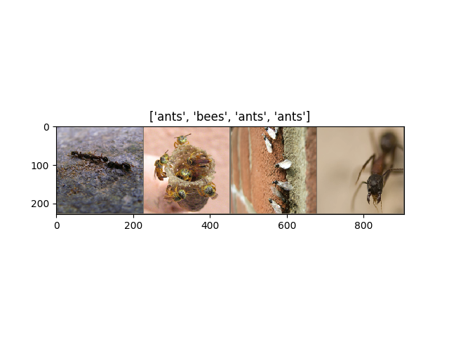
可视化一些图像|
让我们可视化一些训练图像,以便了解数据扩增。
def imshow(inp, title=None):
    """Imshow for Tensor."""
    inp = inp.numpy().transpose((1, 2, 0))
    mean = np.array([0.485, 0.456, 0.406])
    std = np.array([0.229, 0.224, 0.225])
    inp = std * inp + mean
    inp = np.clip(inp, 0, 1)
    plt.imshow(inp)
    if title is not None:
        plt.title(title)
    plt.pause(0.001)  # pause a bit so that plots are updated


# Get a batch of training data
inputs, classes = next(iter(dataloaders['train']))

# Make a grid from batch
out = torchvision.utils.make_grid(inputs)

imshow(out, title=[class_names[x] for x in classes])
训练模型|
现在,让我们编写一个通用函数来训练模型。 在这里,我们将说明:
调整学习率
保存最佳模型
下面的参数scheduler是一个来自torch.optim.lr_scheduler的 LR 调度器对象。
def train_model(model, criterion, optimizer, scheduler, num_epochs=25):
    since = time.time()

    best_model_wts = copy.deepcopy(model.state_dict())
    best_acc = 0.0

    for epoch in range(num_epochs):
        print('Epoch {}/{}'.format(epoch, num_epochs - 1))
        print('-' * 10)

        # Each epoch has a training and validation phase
        for phase in ['train', 'val']:
            if phase == 'train':
                model.train()  # Set model to training mode
            else:
                model.eval()   # Set model to evaluate mode

            running_loss = 0.0
            running_corrects = 0

            # Iterate over data.
            for inputs, labels in dataloaders[phase]:
                inputs = inputs.to(device)
                labels = labels.to(device)

                # zero the parameter gradients
                optimizer.zero_grad()

                # forward
                # track history if only in train
                with torch.set_grad_enabled(phase == 'train'):
                    outputs = model(inputs)
                    _, preds = torch.max(outputs, 1)
                    loss = criterion(outputs, labels)

                    # backward + optimize only if in training phase
                    if phase == 'train':
                        loss.backward()
                        optimizer.step()

                # statistics
                running_loss += loss.item() * inputs.size(0)
                running_corrects += torch.sum(preds == labels.data)
            if phase == 'train':
                scheduler.step()

            epoch_loss = running_loss / dataset_sizes[phase]
            epoch_acc = running_corrects.double() / dataset_sizes[phase]

            print('{} Loss: {:.4f} Acc: {:.4f}'.format(
                phase, epoch_loss, epoch_acc))

            # deep copy the model
            if phase == 'val' and epoch_acc > best_acc:
                best_acc = epoch_acc
                best_model_wts = copy.deepcopy(model.state_dict())

        print()

    time_elapsed = time.time() - since
    print('Training complete in {:.0f}m {:.0f}s'.format(
        time_elapsed // 60, time_elapsed % 60))
    print('Best val Acc: {:4f}'.format(best_acc))

    # load best model weights
    model.load_state_dict(best_model_wts)
    return model
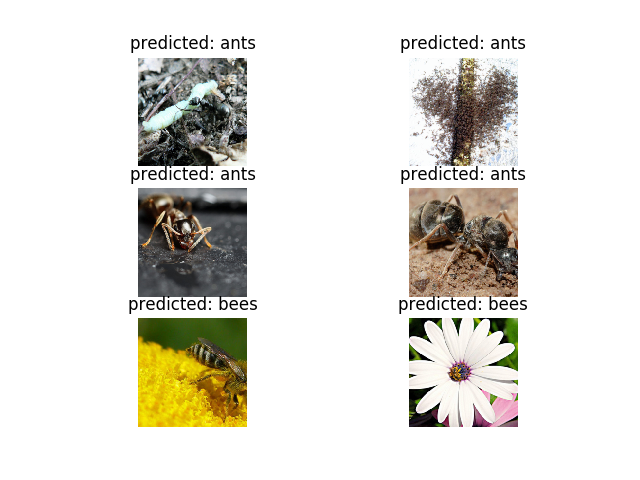
可视化模型预测|
用于显示几个图像的预测的通用函数
def visualize_model(model, num_images=6):
    was_training = model.training
    model.eval()
    images_so_far = 0
    fig = plt.figure()

    with torch.no_grad():
        for i, (inputs, labels) in enumerate(dataloaders['val']):
            inputs = inputs.to(device)
            labels = labels.to(device)

            outputs = model(inputs)
            _, preds = torch.max(outputs, 1)

            for j in range(inputs.size()[0]):
                images_so_far += 1
                ax = plt.subplot(num_images//2, 2, images_so_far)
                ax.axis('off')
                ax.set_title('predicted: {}'.format(class_names[preds[j]]))
                imshow(inputs.cpu().data[j])

                if images_so_far == num_images:
                    model.train(mode=was_training)
                    return
        model.train(mode=was_training)
微调convnet
加载预训练模型并重置最后的全连接层。
model_ft = models.resnet18(pretrained=True)
num_ftrs = model_ft.fc.in_features
# Here the size of each output sample is set to 2.
# Alternatively, it can be generalized to nn.Linear(num_ftrs, len(class_names)).
model_ft.fc = nn.Linear(num_ftrs, 2)

model_ft = model_ft.to(device)

criterion = nn.CrossEntropyLoss()

# Observe that all parameters are being optimized
optimizer_ft = optim.SGD(model_ft.parameters(), lr=0.001, momentum=0.9)

# Decay LR by a factor of 0.1 every 7 epochs
exp_lr_scheduler = lr_scheduler.StepLR(optimizer_ft, step_size=7, gamma=0.1)
训练和评估
在 CPU 大约需要 15-25 分钟。 在 GPU 上,它只需不到一分钟。
model_ft = train_model(model_ft, criterion, optimizer_ft, exp_lr_scheduler,
                       num_epochs=25)
输出:
Epoch 0/24
----------
train Loss: 0.6393 Acc: 0.6885
val Loss: 0.2587 Acc: 0.9085

Epoch 1/24
----------
train Loss: 0.4556 Acc: 0.8115
val Loss: 0.2912 Acc: 0.8758

Epoch 2/24
----------
train Loss: 0.6616 Acc: 0.7623
val Loss: 0.4153 Acc: 0.8562

Epoch 3/24
----------
train Loss: 0.4349 Acc: 0.8402
val Loss: 0.3520 Acc: 0.8627

Epoch 4/24
----------
train Loss: 0.5696 Acc: 0.7910
val Loss: 0.2692 Acc: 0.8889

Epoch 5/24
----------
train Loss: 0.5294 Acc: 0.8197
val Loss: 0.5651 Acc: 0.8105

Epoch 6/24
----------
train Loss: 0.6484 Acc: 0.7623
val Loss: 0.2850 Acc: 0.8758

Epoch 7/24
----------
train Loss: 0.3637 Acc: 0.8156
val Loss: 0.2712 Acc: 0.8954

Epoch 8/24
----------
train Loss: 0.4995 Acc: 0.7828
val Loss: 0.2427 Acc: 0.8954

Epoch 9/24
----------
train Loss: 0.3242 Acc: 0.8648
val Loss: 0.2123 Acc: 0.9281

Epoch 10/24
----------
train Loss: 0.2764 Acc: 0.9016
val Loss: 0.1926 Acc: 0.9346

Epoch 11/24
----------
train Loss: 0.3109 Acc: 0.8443
val Loss: 0.2014 Acc: 0.9412

Epoch 12/24
----------
train Loss: 0.3170 Acc: 0.8607
val Loss: 0.1852 Acc: 0.9346

Epoch 13/24
----------
train Loss: 0.2991 Acc: 0.8811
val Loss: 0.1994 Acc: 0.9346

Epoch 14/24
----------
train Loss: 0.2694 Acc: 0.8770
val Loss: 0.1886 Acc: 0.9346

Epoch 15/24
----------
train Loss: 0.3005 Acc: 0.8607
val Loss: 0.1910 Acc: 0.9346

Epoch 16/24
----------
train Loss: 0.2447 Acc: 0.8893
val Loss: 0.1954 Acc: 0.9150

Epoch 17/24
----------
train Loss: 0.3324 Acc: 0.8689
val Loss: 0.2152 Acc: 0.9281

Epoch 18/24
----------
train Loss: 0.2918 Acc: 0.8566
val Loss: 0.1869 Acc: 0.9346

Epoch 19/24
----------
train Loss: 0.2623 Acc: 0.8730
val Loss: 0.1865 Acc: 0.9281

Epoch 20/24
----------
train Loss: 0.2750 Acc: 0.8770
val Loss: 0.1858 Acc: 0.9477

Epoch 21/24
----------
train Loss: 0.3313 Acc: 0.8770
val Loss: 0.1775 Acc: 0.9346

Epoch 22/24
----------
train Loss: 0.3713 Acc: 0.8320
val Loss: 0.1760 Acc: 0.9477

Epoch 23/24
----------
train Loss: 0.2388 Acc: 0.9016
val Loss: 0.2120 Acc: 0.9346

Epoch 24/24
----------
train Loss: 0.2843 Acc: 0.8852
val Loss: 0.1914 Acc: 0.9412

Training complete in 7m 12s
Best val Acc: 0.947712
visualize_model(model_ft)
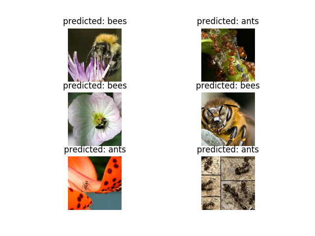
作为固定特征提取器的 ConvNet
在这里,我们需要冻结除最后一层之外的所有网络。 我们需要设置requires_grad = False来冻结参数,以便渐变不会以backward()
你可以在这里的文档中阅读更多关于此内容。
model_conv = torchvision.models.resnet18(pretrained=True)
for param in model_conv.parameters():
    param.requires_grad = False

# Parameters of newly constructed modules have requires_grad=True by default
num_ftrs = model_conv.fc.in_features
model_conv.fc = nn.Linear(num_ftrs, 2)

model_conv = model_conv.to(device)

criterion = nn.CrossEntropyLoss()

# Observe that only parameters of final layer are being optimized as
# opposed to before.
optimizer_conv = optim.SGD(model_conv.fc.parameters(), lr=0.001, momentum=0.9)

# Decay LR by a factor of 0.1 every 7 epochs
exp_lr_scheduler = lr_scheduler.StepLR(optimizer_conv, step_size=7, gamma=0.1)
训练和评估
在 CPU 上,与以前的方案相比,这大约需要一半的时间。 这是符合预期的,因为网络的大部分不需要计算梯度。 但是,需要前向计算。
model_conv = train_model(model_conv, criterion, optimizer_conv,
                         exp_lr_scheduler, num_epochs=25)
输出:
Epoch 0/24
----------
train Loss: 0.7926 Acc: 0.5943
val Loss: 0.5578 Acc: 0.7190

Epoch 1/24
----------
train Loss: 0.5976 Acc: 0.7336
val Loss: 0.1815 Acc: 0.9412

Epoch 2/24
----------
train Loss: 0.4328 Acc: 0.8033
val Loss: 0.1525 Acc: 0.9542

Epoch 3/24
----------
train Loss: 0.4571 Acc: 0.7951
val Loss: 0.1954 Acc: 0.9542

Epoch 4/24
----------
train Loss: 0.3612 Acc: 0.8689
val Loss: 0.2218 Acc: 0.9477

Epoch 5/24
----------
train Loss: 0.3450 Acc: 0.8402
val Loss: 0.1588 Acc: 0.9477

Epoch 6/24
----------
train Loss: 0.4848 Acc: 0.7623
val Loss: 0.1979 Acc: 0.9477

Epoch 7/24
----------
train Loss: 0.4575 Acc: 0.8033
val Loss: 0.1580 Acc: 0.9477

Epoch 8/24
----------
train Loss: 0.3402 Acc: 0.8730
val Loss: 0.1731 Acc: 0.9542

Epoch 9/24
----------
train Loss: 0.2688 Acc: 0.8811
val Loss: 0.1669 Acc: 0.9477

Epoch 10/24
----------
train Loss: 0.3437 Acc: 0.8443
val Loss: 0.1609 Acc: 0.9477

Epoch 11/24
----------
train Loss: 0.3340 Acc: 0.8689
val Loss: 0.1569 Acc: 0.9477

Epoch 12/24
----------
train Loss: 0.3102 Acc: 0.8730
val Loss: 0.1737 Acc: 0.9542

Epoch 13/24
----------
train Loss: 0.3481 Acc: 0.8443
val Loss: 0.1630 Acc: 0.9542

Epoch 14/24
----------
train Loss: 0.3166 Acc: 0.8525
val Loss: 0.2027 Acc: 0.9281

Epoch 15/24
----------
train Loss: 0.3047 Acc: 0.8770
val Loss: 0.1743 Acc: 0.9542

Epoch 16/24
----------
train Loss: 0.3283 Acc: 0.8566
val Loss: 0.2201 Acc: 0.9281

Epoch 17/24
----------
train Loss: 0.3940 Acc: 0.8402
val Loss: 0.1738 Acc: 0.9477

Epoch 18/24
----------
train Loss: 0.3730 Acc: 0.8197
val Loss: 0.1747 Acc: 0.9542

Epoch 19/24
----------
train Loss: 0.3033 Acc: 0.8443
val Loss: 0.1535 Acc: 0.9542

Epoch 20/24
----------
train Loss: 0.3816 Acc: 0.8320
val Loss: 0.1737 Acc: 0.9542

Epoch 21/24
----------
train Loss: 0.3424 Acc: 0.8566
val Loss: 0.1567 Acc: 0.9477

Epoch 22/24
----------
train Loss: 0.2936 Acc: 0.8730
val Loss: 0.1579 Acc: 0.9477

Epoch 23/24
----------
train Loss: 0.3403 Acc: 0.8525
val Loss: 0.1576 Acc: 0.9542

Epoch 24/24
----------
train Loss: 0.3017 Acc: 0.8443
val Loss: 0.1566 Acc: 0.9477

Training complete in 3m 17s
Best val Acc: 0.954248
visualize_model(model_conv)

plt.ioff()
plt.show()