[TOC]
An embedding is a mapping from discrete objects, such as words, to vectors of real numbers. For example, a 300-dimensional embedding for English words could include:
blue:  (0.01359, 0.00075997, 0.24608, ..., -0.2524, 1.0048, 0.06259)
blues:  (0.01396, 0.11887, -0.48963, ..., 0.033483, -0.10007, 0.1158)
orange:  (-0.24776, -0.12359, 0.20986, ..., 0.079717, 0.23865, -0.014213)
oranges:  (-0.35609, 0.21854, 0.080944, ..., -0.35413, 0.38511, -0.070976)
Embeddings let you apply machine learning to discrete inputs. Classifiers, and neural networks more generally, are designed to work with dense continuous vectors, where all values contribute to define what an object is. If discrete objects are naively encoded as discrete atoms, e.g., unique id numbers, they hinder learning and generalization. One way to think of embeddings is as a way to transform non-vector objects into useful inputs for machine learning.
Embeddings are also useful as outputs of machine learning. Because embeddings map objects to vectors, applications can use similarity in vector space (e.g., Euclidean distance or the angle between vectors) as a robust and flexible measure of object similarity. One common use is to find nearest neighbors. Using the same word embeddings above, for instance, here are the three nearest neighbors for each word and the corresponding angles (in degrees):
blue:  (red, 47.6°), (yellow, 51.9°), (purple, 52.4°)
blues:  (jazz, 53.3°), (folk, 59.1°), (bluegrass, 60.6°)
orange:  (yellow, 53.5°), (colored, 58.0°), (bright, 59.9°)
oranges:  (apples, 45.3°), (lemons, 48.3°), (mangoes, 50.4°)
This would tell an application that apples and oranges are in some way more similar (45.3° apart) than lemons and oranges (48.3° apart).
To train word embeddings in TensorFlow, we first need to split the text into words and assign an integer to every word in the vocabulary. Let us assume that this has already been done, and that word_ids is a vector of these integers. For example, the sentence “I have a cat.” could be split into [“I”, “have”, “a”, “cat”, “.”] and then the corresponding word_ids tensor would have shape [5] and consist of 5 integers. To get these word ids embedded, we need to create the embedding variable and use the tf.gather function as follows:
word_embeddings = tf.get_variable(“word_embeddings”,
    [vocabulary_size, embedding_size])
embedded_word_ids = tf.gather(word_embeddings, word_ids)
After this, the tensor embedded_word_ids will have shape [5, embedding_size] in our example and contain the embeddings (dense vectors) for each of the 5 words. The variable word_embeddings will be learned and at the end of the training it will contain the embeddings for all words in the vocabulary. The embeddings can be trained in many ways, depending on the data available. For example, one could use a recurrent neural network to predict the next word from the previous one given a large corpus of sentences, or one could train two networks to do multi-lingual translation. These methods are described in Vector Representations of Words tutorial, but in all cases there is an embedding variable like above and words are embedded using tf.gather, as shown.
TensorBoard has a built-in visualizer, called the Embedding Projector, for interactive visualization of embeddings. The embedding projector will read the embeddings from your checkpoint file and project them into 3 dimensions using principal component analysis. For a visual explanation of PCA, see this article. Another very useful projection you can use is t-SNE.
If you are working with an embedding, you'll probably want to attach labels/images to the data points. You can do this by generating a metadata file containing the labels for each point and configuring the projector either by using our Python API, or manually constructing and saving a projector_config.pbtxt in the same directory as your checkpoint file.
For in depth information on how to run TensorBoard and make sure you are logging all the necessary information, see TensorBoard: Visualizing Learning.
To visualize your embeddings, there are 3 things you need to do:
embedding_var = tf.get_variable(....)LOG_DIR.saver = tf.train.Saver()
saver.save(session, os.path.join(LOG_DIR, "model.ckpt"), step)If you have any metadata (labels, images) associated with your embedding, you can tell TensorBoard about it either by directly storing a projector_config.pbtxt in the LOG_DIR, or use our python API.
For instance, the following projector_config.ptxt associates the word_embedding tensor with metadata stored in $LOG_DIR/metadata.tsv:
embeddings {
  tensor_name: 'word_embedding'
  metadata_path: '$LOG_DIR/metadata.tsv'
}
The same config can be produced programmatically using the following code snippet:
from tensorflow.contrib.tensorboard.plugins import projector

# Create randomly initialized embedding weights which will be trained.
vocabulary_size = 10000
embedding_size = 200
embedding_var = tf.get_variable('word_embedding', [vocabulary_size, embedding_size])

# Format: tensorflow/tensorboard/plugins/projector/projector_config.proto
config = projector.ProjectorConfig()

# You can add multiple embeddings. Here we add only one.
embedding = config.embeddings.add()
embedding.tensor_name = embedding_var.name
# Link this tensor to its metadata file (e.g. labels).
embedding.metadata_path = os.path.join(LOG_DIR, 'metadata.tsv')

# Use the same LOG_DIR where you stored your checkpoint.
summary_writer = tf.summary.FileWriter(LOG_DIR)

# The next line writes a projector_config.pbtxt in the LOG_DIR. TensorBoard will
# read this file during startup.
projector.visualize_embeddings(summary_writer, config)
After running your model and training your embeddings, run TensorBoard and point it to the LOG_DIR of the job.
tensorboard --logdir=LOG_DIRThen click on the Embeddings tab on the top pane and select the appropriate run (if there are more than one run).
Usually embeddings have metadata associated with it (e.g. labels, images). The metadata should be stored in a separate file outside of the model checkpoint since the metadata is not a trainable parameter of the model. The format should be a TSV file (tab characters shown in red) with the first line containing column headers (shown in bold) and subsequent lines contain the metadata values:
 WordFrequency
 Airplane345
 Car241
 ...
There is no explicit key shared with the main data file; instead, the order in the metadata file is assumed to match the order in the embedding tensor. In other words, the first line is the header information and the (i+1)-th line in the metadata file corresponds to the i-th row of the embedding tensor stored in the checkpoint.
Note: If the TSV metadata file has only a single column, then we don’t expect a header row, and assume each row is the label of the embedding. We include this exception because it matches the commonly-used "vocab file" format.
If you have images associated with your embeddings, you will need to produce a single image consisting of small thumbnails of each data point. This is known as the sprite image. The sprite should have the same number of rows and columns with thumbnails stored in row-first order: the first data point placed in the top left and the last data point in the bottom right:
| 0 | 1 | 2 |
| 3 | 4 | 5 |
| 6 | 7 |
Note in the example above that the last row doesn't have to be filled. For a concrete example of a sprite, see this sprite image of 10,000 MNIST digits (100x100).
Note: We currently support sprites up to 8192px X 8192px.
After constructing the sprite, you need to tell the Embedding Projector where to find it:
embedding.sprite.image_path = PATH_TO_SPRITE_IMAGE
# Specify the width and height of a single thumbnail.
embedding.sprite.single_image_dim.extend([w, h])The Embedding Projector has three panels:
The Embedding Projector has three methods of reducing the dimensionality of a data set: two linear and one nonlinear. Each method can be used to create either a two- or three-dimensional view.
Principal Component Analysis A straightforward technique for reducing dimensions is Principal Component Analysis (PCA). The Embedding Projector computes the top 10 principal components. The menu lets you project those components onto any combination of two or three. PCA is a linear projection, often effective at examining global geometry.
t-SNE A popular non-linear dimensionality reduction technique is t-SNE. The Embedding Projector offers both two- and three-dimensional t-SNE views. Layout is performed client-side animating every step of the algorithm. Because t-SNE often preserves some local structure, it is useful for exploring local neighborhoods and finding clusters. Although extremely useful for visualizing high-dimensional data, t-SNE plots can sometimes be mysterious or misleading. See this great article for how to use t-SNE effectively.
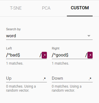
Custom You can also construct specialized linear projections based on text searches for finding meaningful directions in space. To define a projection axis, enter two search strings or regular expressions. The program computes the centroids of the sets of points whose labels match these searches, and uses the difference vector between centroids as a projection axis.
To explore a data set, you can navigate the views in either a 2D or a 3D mode, zooming, rotating, and panning using natural click-and-drag gestures. Clicking on a point causes the right pane to show an explicit textual list of nearest neighbors, along with distances to the current point. The nearest-neighbor points themselves are highlighted on the projection.
Zooming into the cluster gives some information, but it is sometimes more helpful to restrict the view to a subset of points and perform projections only on those points. To do so, you can select points in multiple ways:
After selecting a set of points, you can isolate those points for further analysis on their own with the "Isolate Points" button in the Inspector pane on the right hand side.
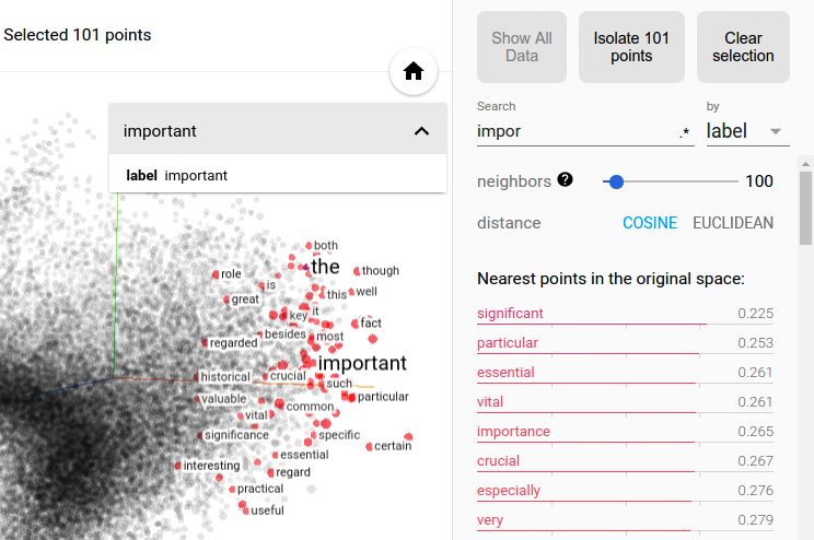
 Selection of the nearest neighbors of “important” in a word embedding dataset.
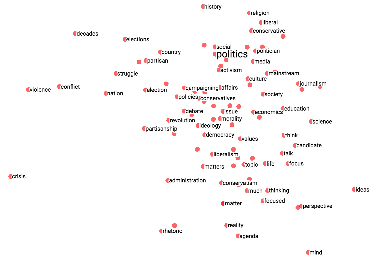
The combination of filtering with custom projection can be powerful. Below, we filtered the 100 nearest neighbors of “politics” and projected them onto the “best” - “worst” vector as an x axis. The y axis is random.
You can see that on the right side we have “ideas”, “science”, “perspective”, “journalism” while on the left we have “crisis”, “violence” and “conflict”.

|

|
| Custom projection controls. | Custom projection of neighbors of "politics" onto "best" - "worst" vector. |
To share your findings, you can use the bookmark panel in the bottom right corner and save the current state (including computed coordinates of any projection) as a small file. The Projector can then be pointed to a set of one or more of these files, producing the panel below. Other users can then walk through a sequence of bookmarks.

Is "embedding" an action or a thing? Both. People talk about embedding words in a vector space (action) and about producing word embeddings (things). Common to both is the notion of embedding as a mapping from discrete objects to vectors. Creating or applying that mapping is an action, but the mapping itself is a thing.
Are embeddings high-dimensional or low-dimensional? It depends. A 300-dimensional vector space of words and phrases, for instance, is often called low-dimensional (and dense) when compared to the millions of words and phrases it can contain. But mathematically it is high-dimensional, displaying many properties that are dramatically different from what our human intuition has learned about 2- and 3-dimensional spaces.
Is an embedding the same as an embedding layer? No; an embedding layer is a part of neural network, but an embedding is a more general concept.