10 Minutes to pandas
This is a short introduction to pandas, geared mainly for new users. 您可以在Cookbook中查看更复杂的配方。
Customarily, we import as follows:
In [1]: import pandas as pd

In [2]: import numpy as np

In [3]: import matplotlib.pyplot as plt
对象创建
See the Data Structure Intro section.
Creating a Series by passing a list of values, letting pandas create
a default integer index:
In [4]: s = pd.Series([1,3,5,np.nan,6,8])

In [5]: s
Out[5]:
0    1.0
1    3.0
2    5.0
3    NaN
4    6.0
5    8.0
dtype: float64
通过传递带有日期时间索引和标记列的NumPy数组来创建DataFrame:
In [6]: dates = pd.date_range('20130101', periods=6)

In [7]: dates
Out[7]:
DatetimeIndex(['2013-01-01', '2013-01-02', '2013-01-03', '2013-01-04',
               '2013-01-05', '2013-01-06'],
              dtype='datetime64[ns]', freq='D')

In [8]: df = pd.DataFrame(np.random.randn(6,4), index=dates, columns=list('ABCD'))

In [9]: df
Out[9]:
                   A         B         C         D
2013-01-01  0.469112 -0.282863 -1.509059 -1.135632
2013-01-02  1.212112 -0.173215  0.119209 -1.044236
2013-01-03 -0.861849 -2.104569 -0.494929  1.071804
2013-01-04  0.721555 -0.706771 -1.039575  0.271860
2013-01-05 -0.424972  0.567020  0.276232 -1.087401
2013-01-06 -0.673690  0.113648 -1.478427  0.524988
Creating a DataFrame by passing a dict of objects that can be converted to series-like.
In [10]: df2 = pd.DataFrame({ 'A' : 1.,
   ....:                      'B' : pd.Timestamp('20130102'),
   ....:                      'C' : pd.Series(1,index=list(range(4)),dtype='float32'),
   ....:                      'D' : np.array([3] * 4,dtype='int32'),
   ....:                      'E' : pd.Categorical(["test","train","test","train"]),
   ....:                      'F' : 'foo' })
   ....:

In [11]: df2
Out[11]:
     A          B    C  D      E    F
0  1.0 2013-01-02  1.0  3   test  foo
1  1.0 2013-01-02  1.0  3  train  foo
2  1.0 2013-01-02  1.0  3   test  foo
3  1.0 2013-01-02  1.0  3  train  foo
The columns of the resulting DataFrame have different
dtypes.
In [12]: df2.dtypes
Out[12]:
A           float64
B    datetime64[ns]
C           float32
D             int32
E          category
F            object
dtype: object
如果您正在使用IPython,则会自动启用列名称(以及公共属性)的选项卡完成。 以下是将要完成的属性的子集:
In [13]: df2.<TAB>
df2.A                  df2.bool
df2.abs                df2.boxplot
df2.add                df2.C
df2.add_prefix         df2.clip
df2.add_suffix         df2.clip_lower
df2.align              df2.clip_upper
df2.all                df2.columns
df2.any                df2.combine
df2.append             df2.combine_first
df2.apply              df2.compound
df2.applymap           df2.consolidate
df2.D
如您所见,列A,B,C和D会自动完成选项卡。 E也有;为简洁起见,其他属性已被截断。
Viewing Data
See the Basics section.
Here is how to view the top and bottom rows of the frame:
In [14]: df.head()
Out[14]:
                   A         B         C         D
2013-01-01  0.469112 -0.282863 -1.509059 -1.135632
2013-01-02  1.212112 -0.173215  0.119209 -1.044236
2013-01-03 -0.861849 -2.104569 -0.494929  1.071804
2013-01-04  0.721555 -0.706771 -1.039575  0.271860
2013-01-05 -0.424972  0.567020  0.276232 -1.087401

In [15]: df.tail(3)
Out[15]:
                   A         B         C         D
2013-01-04  0.721555 -0.706771 -1.039575  0.271860
2013-01-05 -0.424972  0.567020  0.276232 -1.087401
2013-01-06 -0.673690  0.113648 -1.478427  0.524988
显示索引,列和基础NumPy数据:
In [16]: df.index
Out[16]:
DatetimeIndex(['2013-01-01', '2013-01-02', '2013-01-03', '2013-01-04',
               '2013-01-05', '2013-01-06'],
              dtype='datetime64[ns]', freq='D')

In [17]: df.columns
Out[17]: Index(['A', 'B', 'C', 'D'], dtype='object')

In [18]: df.values
Out[18]:
array([[ 0.4691, -0.2829, -1.5091, -1.1356],
       [ 1.2121, -0.1732,  0.1192, -1.0442],
       [-0.8618, -2.1046, -0.4949,  1.0718],
       [ 0.7216, -0.7068, -1.0396,  0.2719],
       [-0.425 ,  0.567 ,  0.2762, -1.0874],
       [-0.6737,  0.1136, -1.4784,  0.525 ]])
describe()显示数据的快速统计摘要:
In [19]: df.describe()
Out[19]:
              A         B         C         D
count  6.000000  6.000000  6.000000  6.000000
mean   0.073711 -0.431125 -0.687758 -0.233103
std    0.843157  0.922818  0.779887  0.973118
min   -0.861849 -2.104569 -1.509059 -1.135632
25%   -0.611510 -0.600794 -1.368714 -1.076610
50%    0.022070 -0.228039 -0.767252 -0.386188
75%    0.658444  0.041933 -0.034326  0.461706
max    1.212112  0.567020  0.276232  1.071804
Transposing your data:
In [20]: df.T
Out[20]:
   2013-01-01  2013-01-02  2013-01-03  2013-01-04  2013-01-05  2013-01-06
A    0.469112    1.212112   -0.861849    0.721555   -0.424972   -0.673690
B   -0.282863   -0.173215   -2.104569   -0.706771    0.567020    0.113648
C   -1.509059    0.119209   -0.494929   -1.039575    0.276232   -1.478427
D   -1.135632   -1.044236    1.071804    0.271860   -1.087401    0.524988
Sorting by an axis:
In [21]: df.sort_index(axis=1, ascending=False)
Out[21]:
                   D         C         B         A
2013-01-01 -1.135632 -1.509059 -0.282863  0.469112
2013-01-02 -1.044236  0.119209 -0.173215  1.212112
2013-01-03  1.071804 -0.494929 -2.104569 -0.861849
2013-01-04  0.271860 -1.039575 -0.706771  0.721555
2013-01-05 -1.087401  0.276232  0.567020 -0.424972
2013-01-06  0.524988 -1.478427  0.113648 -0.673690
Sorting by values:
In [22]: df.sort_values(by='B')
Out[22]:
                   A         B         C         D
2013-01-03 -0.861849 -2.104569 -0.494929  1.071804
2013-01-04  0.721555 -0.706771 -1.039575  0.271860
2013-01-01  0.469112 -0.282863 -1.509059 -1.135632
2013-01-02  1.212112 -0.173215  0.119209 -1.044236
2013-01-06 -0.673690  0.113648 -1.478427  0.524988
2013-01-05 -0.424972  0.567020  0.276232 -1.087401
Selection
Note
While standard Python / Numpy expressions for selecting and setting are
intuitive and come in handy for interactive work, for production code, we
recommend the optimized pandas data access methods, .at, .iat,
.loc and .iloc.
See the indexing documentation Indexing and Selecting Data and MultiIndex / Advanced Indexing.
Getting
Selecting a single column, which yields a Series,
equivalent to df.A:
In [23]: df['A']
Out[23]:
2013-01-01    0.469112
2013-01-02    1.212112
2013-01-03   -0.861849
2013-01-04    0.721555
2013-01-05   -0.424972
2013-01-06   -0.673690
Freq: D, Name: A, dtype: float64
Selecting via [], which slices the rows.
In [24]: df[0:3]
Out[24]:
                   A         B         C         D
2013-01-01  0.469112 -0.282863 -1.509059 -1.135632
2013-01-02  1.212112 -0.173215  0.119209 -1.044236
2013-01-03 -0.861849 -2.104569 -0.494929  1.071804

In [25]: df['20130102':'20130104']
Out[25]:
                   A         B         C         D
2013-01-02  1.212112 -0.173215  0.119209 -1.044236
2013-01-03 -0.861849 -2.104569 -0.494929  1.071804
2013-01-04  0.721555 -0.706771 -1.039575  0.271860
Selection by Label
See more in Selection by Label.
For getting a cross section using a label:
In [26]: df.loc[dates[0]]
Out[26]:
A    0.469112
B   -0.282863
C   -1.509059
D   -1.135632
Name: 2013-01-01 00:00:00, dtype: float64
Selecting on a multi-axis by label:
In [27]: df.loc[:,['A','B']]
Out[27]:
                   A         B
2013-01-01  0.469112 -0.282863
2013-01-02  1.212112 -0.173215
2013-01-03 -0.861849 -2.104569
2013-01-04  0.721555 -0.706771
2013-01-05 -0.424972  0.567020
2013-01-06 -0.673690  0.113648
Showing label slicing, both endpoints are included:
In [28]: df.loc['20130102':'20130104',['A','B']]
Out[28]:
                   A         B
2013-01-02  1.212112 -0.173215
2013-01-03 -0.861849 -2.104569
2013-01-04  0.721555 -0.706771
Reduction in the dimensions of the returned object:
In [29]: df.loc['20130102',['A','B']]
Out[29]:
A    1.212112
B   -0.173215
Name: 2013-01-02 00:00:00, dtype: float64
For getting a scalar value:
In [30]: df.loc[dates[0],'A']
Out[30]: 0.46911229990718628
For getting fast access to a scalar (equivalent to the prior method):
In [31]: df.at[dates[0],'A']
Out[31]: 0.46911229990718628
Selection by Position
See more in Selection by Position.
Select via the position of the passed integers:
In [32]: df.iloc[3]
Out[32]:
A    0.721555
B   -0.706771
C   -1.039575
D    0.271860
Name: 2013-01-04 00:00:00, dtype: float64
By integer slices, acting similar to numpy/python:
In [33]: df.iloc[3:5,0:2]
Out[33]:
                   A         B
2013-01-04  0.721555 -0.706771
2013-01-05 -0.424972  0.567020
By lists of integer position locations, similar to the numpy/python style:
In [34]: df.iloc[[1,2,4],[0,2]]
Out[34]:
                   A         C
2013-01-02  1.212112  0.119209
2013-01-03 -0.861849 -0.494929
2013-01-05 -0.424972  0.276232
For slicing rows explicitly:
In [35]: df.iloc[1:3,:]
Out[35]:
                   A         B         C         D
2013-01-02  1.212112 -0.173215  0.119209 -1.044236
2013-01-03 -0.861849 -2.104569 -0.494929  1.071804
For slicing columns explicitly:
In [36]: df.iloc[:,1:3]
Out[36]:
                   B         C
2013-01-01 -0.282863 -1.509059
2013-01-02 -0.173215  0.119209
2013-01-03 -2.104569 -0.494929
2013-01-04 -0.706771 -1.039575
2013-01-05  0.567020  0.276232
2013-01-06  0.113648 -1.478427
For getting a value explicitly:
In [37]: df.iloc[1,1]
Out[37]: -0.17321464905330858
For getting fast access to a scalar (equivalent to the prior method):
In [38]: df.iat[1,1]
Out[38]: -0.17321464905330858
Boolean Indexing
Using a single column’s values to select data.
In [39]: df[df.A > 0]
Out[39]:
                   A         B         C         D
2013-01-01  0.469112 -0.282863 -1.509059 -1.135632
2013-01-02  1.212112 -0.173215  0.119209 -1.044236
2013-01-04  0.721555 -0.706771 -1.039575  0.271860
Selecting values from a DataFrame where a boolean condition is met.
In [40]: df[df > 0]
Out[40]:
                   A         B         C         D
2013-01-01  0.469112       NaN       NaN       NaN
2013-01-02  1.212112       NaN  0.119209       NaN
2013-01-03       NaN       NaN       NaN  1.071804
2013-01-04  0.721555       NaN       NaN  0.271860
2013-01-05       NaN  0.567020  0.276232       NaN
2013-01-06       NaN  0.113648       NaN  0.524988
Using the isin() method for filtering:
In [41]: df2 = df.copy()

In [42]: df2['E'] = ['one', 'one','two','three','four','three']

In [43]: df2
Out[43]:
                   A         B         C         D      E
2013-01-01  0.469112 -0.282863 -1.509059 -1.135632    one
2013-01-02  1.212112 -0.173215  0.119209 -1.044236    one
2013-01-03 -0.861849 -2.104569 -0.494929  1.071804    two
2013-01-04  0.721555 -0.706771 -1.039575  0.271860  three
2013-01-05 -0.424972  0.567020  0.276232 -1.087401   four
2013-01-06 -0.673690  0.113648 -1.478427  0.524988  three

In [44]: df2[df2['E'].isin(['two','four'])]
Out[44]:
                   A         B         C         D     E
2013-01-03 -0.861849 -2.104569 -0.494929  1.071804   two
2013-01-05 -0.424972  0.567020  0.276232 -1.087401  four
Setting
Setting a new column automatically aligns the data by the indexes.
In [45]: s1 = pd.Series([1,2,3,4,5,6], index=pd.date_range('20130102', periods=6))

In [46]: s1
Out[46]:
2013-01-02    1
2013-01-03    2
2013-01-04    3
2013-01-05    4
2013-01-06    5
2013-01-07    6
Freq: D, dtype: int64

In [47]: df['F'] = s1
Setting values by label:
In [48]: df.at[dates[0],'A'] = 0
Setting values by position:
In [49]: df.iat[0,1] = 0
Setting by assigning with a NumPy array:
In [50]: df.loc[:,'D'] = np.array([5] * len(df))
The result of the prior setting operations.
In [51]: df
Out[51]:
                   A         B         C  D    F
2013-01-01  0.000000  0.000000 -1.509059  5  NaN
2013-01-02  1.212112 -0.173215  0.119209  5  1.0
2013-01-03 -0.861849 -2.104569 -0.494929  5  2.0
2013-01-04  0.721555 -0.706771 -1.039575  5  3.0
2013-01-05 -0.424972  0.567020  0.276232  5  4.0
2013-01-06 -0.673690  0.113648 -1.478427  5  5.0
A where operation with setting.
In [52]: df2 = df.copy()

In [53]: df2[df2 > 0] = -df2

In [54]: df2
Out[54]:
                   A         B         C  D    F
2013-01-01  0.000000  0.000000 -1.509059 -5  NaN
2013-01-02 -1.212112 -0.173215 -0.119209 -5 -1.0
2013-01-03 -0.861849 -2.104569 -0.494929 -5 -2.0
2013-01-04 -0.721555 -0.706771 -1.039575 -5 -3.0
2013-01-05 -0.424972 -0.567020 -0.276232 -5 -4.0
2013-01-06 -0.673690 -0.113648 -1.478427 -5 -5.0
Missing Data
pandas primarily uses the value np.nan to represent missing data. It is by
default not included in computations. See the Missing Data section.
Reindexing allows you to change/add/delete the index on a specified axis. This returns a copy of the data.
In [55]: df1 = df.reindex(index=dates[0:4], columns=list(df.columns) + ['E'])

In [56]: df1.loc[dates[0]:dates[1],'E'] = 1

In [57]: df1
Out[57]:
                   A         B         C  D    F    E
2013-01-01  0.000000  0.000000 -1.509059  5  NaN  1.0
2013-01-02  1.212112 -0.173215  0.119209  5  1.0  1.0
2013-01-03 -0.861849 -2.104569 -0.494929  5  2.0  NaN
2013-01-04  0.721555 -0.706771 -1.039575  5  3.0  NaN
To drop any rows that have missing data.
In [58]: df1.dropna(how='any')
Out[58]:
                   A         B         C  D    F    E
2013-01-02  1.212112 -0.173215  0.119209  5  1.0  1.0
Filling missing data.
In [59]: df1.fillna(value=5)
Out[59]:
                   A         B         C  D    F    E
2013-01-01  0.000000  0.000000 -1.509059  5  5.0  1.0
2013-01-02  1.212112 -0.173215  0.119209  5  1.0  1.0
2013-01-03 -0.861849 -2.104569 -0.494929  5  2.0  5.0
2013-01-04  0.721555 -0.706771 -1.039575  5  3.0  5.0
To get the boolean mask where values are nan.
In [60]: pd.isna(df1)
Out[60]:
                A      B      C      D      F      E
2013-01-01  False  False  False  False   True  False
2013-01-02  False  False  False  False  False  False
2013-01-03  False  False  False  False  False   True
2013-01-04  False  False  False  False  False   True
Operations
See the Basic section on Binary Ops.
Stats
一般操作排除缺失数据。
执行描述性统计:
In [61]: df.mean()
Out[61]:
A   -0.004474
B   -0.383981
C   -0.687758
D    5.000000
F    3.000000
dtype: float64
另一个轴上的操作相同:
In [62]: df.mean(1)
Out[62]:
2013-01-01    0.872735
2013-01-02    1.431621
2013-01-03    0.707731
2013-01-04    1.395042
2013-01-05    1.883656
2013-01-06    1.592306
Freq: D, dtype: float64
使用具有不同维度且需要对齐的对象进行操作。 此外,pandas会自动沿指定维度进行广播。
In [63]: s = pd.Series([1,3,5,np.nan,6,8], index=dates).shift(2)

In [64]: s
Out[64]:
2013-01-01    NaN
2013-01-02    NaN
2013-01-03    1.0
2013-01-04    3.0
2013-01-05    5.0
2013-01-06    NaN
Freq: D, dtype: float64

In [65]: df.sub(s, axis='index')
Out[65]:
                   A         B         C    D    F
2013-01-01       NaN       NaN       NaN  NaN  NaN
2013-01-02       NaN       NaN       NaN  NaN  NaN
2013-01-03 -1.861849 -3.104569 -1.494929  4.0  1.0
2013-01-04 -2.278445 -3.706771 -4.039575  2.0  0.0
2013-01-05 -5.424972 -4.432980 -4.723768  0.0 -1.0
2013-01-06       NaN       NaN       NaN  NaN  NaN
Apply
Applying functions to the data:
In [66]: df.apply(np.cumsum)
Out[66]:
                   A         B         C   D     F
2013-01-01  0.000000  0.000000 -1.509059   5   NaN
2013-01-02  1.212112 -0.173215 -1.389850  10   1.0
2013-01-03  0.350263 -2.277784 -1.884779  15   3.0
2013-01-04  1.071818 -2.984555 -2.924354  20   6.0
2013-01-05  0.646846 -2.417535 -2.648122  25  10.0
2013-01-06 -0.026844 -2.303886 -4.126549  30  15.0

In [67]: df.apply(lambda x: x.max() - x.min())
Out[67]:
A    2.073961
B    2.671590
C    1.785291
D    0.000000
F    4.000000
dtype: float64
Histogramming
See more at Histogramming and Discretization.
In [68]: s = pd.Series(np.random.randint(0, 7, size=10))

In [69]: s
Out[69]:
0    4
1    2
2    1
3    2
4    6
5    4
6    4
7    6
8    4
9    4
dtype: int64

In [70]: s.value_counts()
Out[70]:
4    5
6    2
2    2
1    1
dtype: int64
String Methods
Series is equipped with a set of string processing methods in the str attribute that make it easy to operate on each element of the array, as in the code snippet below. Note that pattern-matching in str generally uses regular expressions by default (and in some cases always uses them). See more at Vectorized String Methods.
In [71]: s = pd.Series(['A', 'B', 'C', 'Aaba', 'Baca', np.nan, 'CABA', 'dog', 'cat'])

In [72]: s.str.lower()
Out[72]:
0       a
1       b
2       c
3    aaba
4    baca
5     NaN
6    caba
7     dog
8     cat
dtype: object
Merge
Concat
pandas provides various facilities for easily combining together Series, DataFrame, and Panel objects with various kinds of set logic for the indexes and relational algebra functionality in the case of join / merge-type operations.
See the Merging section.
Concatenating pandas objects together with concat():
In [73]: df = pd.DataFrame(np.random.randn(10, 4))

In [74]: df
Out[74]:
          0         1         2         3
0 -0.548702  1.467327 -1.015962 -0.483075
1  1.637550 -1.217659 -0.291519 -1.745505
2 -0.263952  0.991460 -0.919069  0.266046
3 -0.709661  1.669052  1.037882 -1.705775
4 -0.919854 -0.042379  1.247642 -0.009920
5  0.290213  0.495767  0.362949  1.548106
6 -1.131345 -0.089329  0.337863 -0.945867
7 -0.932132  1.956030  0.017587 -0.016692
8 -0.575247  0.254161 -1.143704  0.215897
9  1.193555 -0.077118 -0.408530 -0.862495

# break it into pieces
In [75]: pieces = [df[:3], df[3:7], df[7:]]

In [76]: pd.concat(pieces)
Out[76]:
          0         1         2         3
0 -0.548702  1.467327 -1.015962 -0.483075
1  1.637550 -1.217659 -0.291519 -1.745505
2 -0.263952  0.991460 -0.919069  0.266046
3 -0.709661  1.669052  1.037882 -1.705775
4 -0.919854 -0.042379  1.247642 -0.009920
5  0.290213  0.495767  0.362949  1.548106
6 -1.131345 -0.089329  0.337863 -0.945867
7 -0.932132  1.956030  0.017587 -0.016692
8 -0.575247  0.254161 -1.143704  0.215897
9  1.193555 -0.077118 -0.408530 -0.862495
Join
SQL style merges. See the Database style joining section.
In [77]: left = pd.DataFrame({'key': ['foo', 'foo'], 'lval': [1, 2]})

In [78]: right = pd.DataFrame({'key': ['foo', 'foo'], 'rval': [4, 5]})

In [79]: left
Out[79]:
   key  lval
0  foo     1
1  foo     2

In [80]: right
Out[80]:
   key  rval
0  foo     4
1  foo     5

In [81]: pd.merge(left, right, on='key')
Out[81]:
   key  lval  rval
0  foo     1     4
1  foo     1     5
2  foo     2     4
3  foo     2     5
Another example that can be given is:
In [82]: left = pd.DataFrame({'key': ['foo', 'bar'], 'lval': [1, 2]})

In [83]: right = pd.DataFrame({'key': ['foo', 'bar'], 'rval': [4, 5]})

In [84]: left
Out[84]:
   key  lval
0  foo     1
1  bar     2

In [85]: right
Out[85]:
   key  rval
0  foo     4
1  bar     5

In [86]: pd.merge(left, right, on='key')
Out[86]:
   key  lval  rval
0  foo     1     4
1  bar     2     5
Append
Append rows to a dataframe. See the Appending section.
In [87]: df = pd.DataFrame(np.random.randn(8, 4), columns=['A','B','C','D'])

In [88]: df
Out[88]:
          A         B         C         D
0  1.346061  1.511763  1.627081 -0.990582
1 -0.441652  1.211526  0.268520  0.024580
2 -1.577585  0.396823 -0.105381 -0.532532
3  1.453749  1.208843 -0.080952 -0.264610
4 -0.727965 -0.589346  0.339969 -0.693205
5 -0.339355  0.593616  0.884345  1.591431
6  0.141809  0.220390  0.435589  0.192451
7 -0.096701  0.803351  1.715071 -0.708758

In [89]: s = df.iloc[3]

In [90]: df.append(s, ignore_index=True)
Out[90]:
          A         B         C         D
0  1.346061  1.511763  1.627081 -0.990582
1 -0.441652  1.211526  0.268520  0.024580
2 -1.577585  0.396823 -0.105381 -0.532532
3  1.453749  1.208843 -0.080952 -0.264610
4 -0.727965 -0.589346  0.339969 -0.693205
5 -0.339355  0.593616  0.884345  1.591431
6  0.141809  0.220390  0.435589  0.192451
7 -0.096701  0.803351  1.715071 -0.708758
8  1.453749  1.208843 -0.080952 -0.264610
Grouping
By “group by” we are referring to a process involving one or more of the following steps:
- Splitting the data into groups based on some criteria
- Applying a function to each group independently
- Combining the results into a data structure
See the Grouping section.
In [91]: df = pd.DataFrame({'A' : ['foo', 'bar', 'foo', 'bar',
   ....:                           'foo', 'bar', 'foo', 'foo'],
   ....:                    'B' : ['one', 'one', 'two', 'three',
   ....:                           'two', 'two', 'one', 'three'],
   ....:                    'C' : np.random.randn(8),
   ....:                    'D' : np.random.randn(8)})
   ....:

In [92]: df
Out[92]:
     A      B         C         D
0  foo    one -1.202872 -0.055224
1  bar    one -1.814470  2.395985
2  foo    two  1.018601  1.552825
3  bar  three -0.595447  0.166599
4  foo    two  1.395433  0.047609
5  bar    two -0.392670 -0.136473
6  foo    one  0.007207 -0.561757
7  foo  three  1.928123 -1.623033
Grouping and then applying the sum() function to the resulting
groups.
In [93]: df.groupby('A').sum()
Out[93]:
            C        D
A
bar -2.802588  2.42611
foo  3.146492 -0.63958
Grouping by multiple columns forms a hierarchical index, and again we can
apply the sum function.
In [94]: df.groupby(['A','B']).sum()
Out[94]:
                  C         D
A   B
bar one   -1.814470  2.395985
    three -0.595447  0.166599
    two   -0.392670 -0.136473
foo one   -1.195665 -0.616981
    three  1.928123 -1.623033
    two    2.414034  1.600434
Reshaping
See the sections on Hierarchical Indexing and Reshaping.
Stack
In [95]: tuples = list(zip(*[['bar', 'bar', 'baz', 'baz',
   ....:                      'foo', 'foo', 'qux', 'qux'],
   ....:                     ['one', 'two', 'one', 'two',
   ....:                      'one', 'two', 'one', 'two']]))
   ....:

In [96]: index = pd.MultiIndex.from_tuples(tuples, names=['first', 'second'])

In [97]: df = pd.DataFrame(np.random.randn(8, 2), index=index, columns=['A', 'B'])

In [98]: df2 = df[:4]

In [99]: df2
Out[99]:
                     A         B
first second
bar   one     0.029399 -0.542108
      two     0.282696 -0.087302
baz   one    -1.575170  1.771208
      two     0.816482  1.100230
The stack() method “compresses” a level in the DataFrame’s
columns.
In [100]: stacked = df2.stack()

In [101]: stacked
Out[101]:
first  second
bar    one     A    0.029399
               B   -0.542108
       two     A    0.282696
               B   -0.087302
baz    one     A   -1.575170
               B    1.771208
       two     A    0.816482
               B    1.100230
dtype: float64
With a “stacked” DataFrame or Series (having a MultiIndex as the
index), the inverse operation of stack() is
unstack(), which by default unstacks the last level:
In [102]: stacked.unstack()
Out[102]:
                     A         B
first second
bar   one     0.029399 -0.542108
      two     0.282696 -0.087302
baz   one    -1.575170  1.771208
      two     0.816482  1.100230

In [103]: stacked.unstack(1)
Out[103]:
second        one       two
first
bar   A  0.029399  0.282696
      B -0.542108 -0.087302
baz   A -1.575170  0.816482
      B  1.771208  1.100230

In [104]: stacked.unstack(0)
Out[104]:
first          bar       baz
second
one    A  0.029399 -1.575170
       B -0.542108  1.771208
two    A  0.282696  0.816482
       B -0.087302  1.100230
Pivot Tables
See the section on Pivot Tables.
In [105]: df = pd.DataFrame({'A' : ['one', 'one', 'two', 'three'] * 3,
   .....:                    'B' : ['A', 'B', 'C'] * 4,
   .....:                    'C' : ['foo', 'foo', 'foo', 'bar', 'bar', 'bar'] * 2,
   .....:                    'D' : np.random.randn(12),
   .....:                    'E' : np.random.randn(12)})
   .....:

In [106]: df
Out[106]:
        A  B    C         D         E
0     one  A  foo  1.418757 -0.179666
1     one  B  foo -1.879024  1.291836
2     two  C  foo  0.536826 -0.009614
3   three  A  bar  1.006160  0.392149
4     one  B  bar -0.029716  0.264599
5     one  C  bar -1.146178 -0.057409
6     two  A  foo  0.100900 -1.425638
7   three  B  foo -1.035018  1.024098
8     one  C  foo  0.314665 -0.106062
9     one  A  bar -0.773723  1.824375
10    two  B  bar -1.170653  0.595974
11  three  C  bar  0.648740  1.167115
We can produce pivot tables from this data very easily:
In [107]: pd.pivot_table(df, values='D', index=['A', 'B'], columns=['C'])
Out[107]:
C             bar       foo
A     B
one   A -0.773723  1.418757
      B -0.029716 -1.879024
      C -1.146178  0.314665
three A  1.006160       NaN
      B       NaN -1.035018
      C  0.648740       NaN
two   A       NaN  0.100900
      B -1.170653       NaN
      C       NaN  0.536826
Time Series
pandas has simple, powerful, and efficient functionality for performing resampling operations during frequency conversion (e.g., converting secondly data into 5-minutely data). This is extremely common in, but not limited to, financial applications. See the Time Series section.
In [108]: rng = pd.date_range('1/1/2012', periods=100, freq='S')

In [109]: ts = pd.Series(np.random.randint(0, 500, len(rng)), index=rng)

In [110]: ts.resample('5Min').sum()
Out[110]:
2012-01-01    25083
Freq: 5T, dtype: int64
Time zone representation:
In [111]: rng = pd.date_range('3/6/2012 00:00', periods=5, freq='D')

In [112]: ts = pd.Series(np.random.randn(len(rng)), rng)

In [113]: ts
Out[113]:
2012-03-06    0.464000
2012-03-07    0.227371
2012-03-08   -0.496922
2012-03-09    0.306389
2012-03-10   -2.290613
Freq: D, dtype: float64

In [114]: ts_utc = ts.tz_localize('UTC')

In [115]: ts_utc
Out[115]:
2012-03-06 00:00:00+00:00    0.464000
2012-03-07 00:00:00+00:00    0.227371
2012-03-08 00:00:00+00:00   -0.496922
2012-03-09 00:00:00+00:00    0.306389
2012-03-10 00:00:00+00:00   -2.290613
Freq: D, dtype: float64
Converting to another time zone:
In [116]: ts_utc.tz_convert('US/Eastern')
Out[116]:
2012-03-05 19:00:00-05:00    0.464000
2012-03-06 19:00:00-05:00    0.227371
2012-03-07 19:00:00-05:00   -0.496922
2012-03-08 19:00:00-05:00    0.306389
2012-03-09 19:00:00-05:00   -2.290613
Freq: D, dtype: float64
Converting between time span representations:
In [117]: rng = pd.date_range('1/1/2012', periods=5, freq='M')

In [118]: ts = pd.Series(np.random.randn(len(rng)), index=rng)

In [119]: ts
Out[119]:
2012-01-31   -1.134623
2012-02-29   -1.561819
2012-03-31   -0.260838
2012-04-30    0.281957
2012-05-31    1.523962
Freq: M, dtype: float64

In [120]: ps = ts.to_period()

In [121]: ps
Out[121]:
2012-01   -1.134623
2012-02   -1.561819
2012-03   -0.260838
2012-04    0.281957
2012-05    1.523962
Freq: M, dtype: float64

In [122]: ps.to_timestamp()
Out[122]:
2012-01-01   -1.134623
2012-02-01   -1.561819
2012-03-01   -0.260838
2012-04-01    0.281957
2012-05-01    1.523962
Freq: MS, dtype: float64
Converting between period and timestamp enables some convenient arithmetic functions to be used. In the following example, we convert a quarterly frequency with year ending in November to 9am of the end of the month following the quarter end:
In [123]: prng = pd.period_range('1990Q1', '2000Q4', freq='Q-NOV')

In [124]: ts = pd.Series(np.random.randn(len(prng)), prng)

In [125]: ts.index = (prng.asfreq('M', 'e') + 1).asfreq('H', 's') + 9

In [126]: ts.head()
Out[126]:
1990-03-01 09:00   -0.902937
1990-06-01 09:00    0.068159
1990-09-01 09:00   -0.057873
1990-12-01 09:00   -0.368204
1991-03-01 09:00   -1.144073
Freq: H, dtype: float64
Categoricals
pandas can include categorical data in a DataFrame. For full docs, see the
categorical introduction and the API documentation.
In [127]: df = pd.DataFrame({"id":[1,2,3,4,5,6], "raw_grade":['a', 'b', 'b', 'a', 'a', 'e']})
Convert the raw grades to a categorical data type.
In [128]: df["grade"] = df["raw_grade"].astype("category")

In [129]: df["grade"]
Out[129]:
0    a
1    b
2    b
3    a
4    a
5    e
Name: grade, dtype: category
Categories (3, object): [a, b, e]
Rename the categories to more meaningful names (assigning to
Series.cat.categories is inplace!).
In [130]: df["grade"].cat.categories = ["very good", "good", "very bad"]
Reorder the categories and simultaneously add the missing categories (methods under Series
.cat return a new Series by default).
In [131]: df["grade"] = df["grade"].cat.set_categories(["very bad", "bad", "medium", "good", "very good"])

In [132]: df["grade"]
Out[132]:
0    very good
1         good
2         good
3    very good
4    very good
5     very bad
Name: grade, dtype: category
Categories (5, object): [very bad, bad, medium, good, very good]
Sorting is per order in the categories, not lexical order.
In [133]: df.sort_values(by="grade")
Out[133]:
   id raw_grade      grade
5   6         e   very bad
1   2         b       good
2   3         b       good
0   1         a  very good
3   4         a  very good
4   5         a  very good
Grouping by a categorical column also shows empty categories.
In [134]: df.groupby("grade").size()
Out[134]:
grade
very bad     1
bad          0
medium       0
good         2
very good    3
dtype: int64
Plotting
See the Plotting docs.
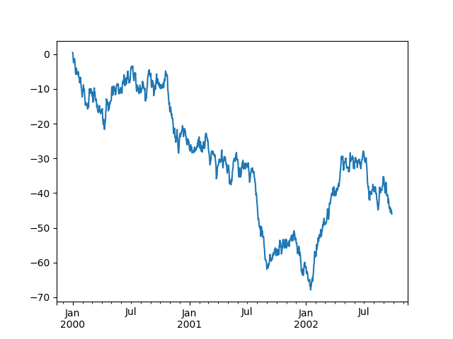
In [135]: ts = pd.Series(np.random.randn(1000), index=pd.date_range('1/1/2000', periods=1000))

In [136]: ts = ts.cumsum()

In [137]: ts.plot()
Out[137]: <matplotlib.axes._subplots.AxesSubplot at 0x7f213444c048>
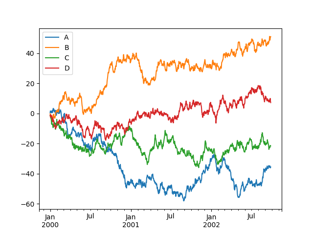
On a DataFrame, the plot() method is a convenience to plot all
of the columns with labels:
In [138]: df = pd.DataFrame(np.random.randn(1000, 4), index=ts.index,
   .....:                   columns=['A', 'B', 'C', 'D'])
   .....:

In [139]: df = df.cumsum()

In [140]: plt.figure(); df.plot(); plt.legend(loc='best')
Out[140]: <matplotlib.legend.Legend at 0x7f212489a780>
Getting Data In/Out
CSV
In [141]: df.to_csv('foo.csv')
In [142]: pd.read_csv('foo.csv')
Out[142]:
     Unnamed: 0          A          B         C          D
0    2000-01-01   0.266457  -0.399641 -0.219582   1.186860
1    2000-01-02  -1.170732  -0.345873  1.653061  -0.282953
2    2000-01-03  -1.734933   0.530468  2.060811  -0.515536
3    2000-01-04  -1.555121   1.452620  0.239859  -1.156896
4    2000-01-05   0.578117   0.511371  0.103552  -2.428202
5    2000-01-06   0.478344   0.449933 -0.741620  -1.962409
6    2000-01-07   1.235339  -0.091757 -1.543861  -1.084753
..          ...        ...        ...       ...        ...
993  2002-09-20 -10.628548  -9.153563 -7.883146  28.313940
994  2002-09-21 -10.390377  -8.727491 -6.399645  30.914107
995  2002-09-22  -8.985362  -8.485624 -4.669462  31.367740
996  2002-09-23  -9.558560  -8.781216 -4.499815  30.518439
997  2002-09-24  -9.902058  -9.340490 -4.386639  30.105593
998  2002-09-25 -10.216020  -9.480682 -3.933802  29.758560
999  2002-09-26 -11.856774 -10.671012 -3.216025  29.369368

[1000 rows x 5 columns]
HDF5
Reading and writing to HDFStores.
Writing to a HDF5 Store.
In [143]: df.to_hdf('foo.h5','df')
Reading from a HDF5 Store.
In [144]: pd.read_hdf('foo.h5','df')
Out[144]:
                    A          B         C          D
2000-01-01   0.266457  -0.399641 -0.219582   1.186860
2000-01-02  -1.170732  -0.345873  1.653061  -0.282953
2000-01-03  -1.734933   0.530468  2.060811  -0.515536
2000-01-04  -1.555121   1.452620  0.239859  -1.156896
2000-01-05   0.578117   0.511371  0.103552  -2.428202
2000-01-06   0.478344   0.449933 -0.741620  -1.962409
2000-01-07   1.235339  -0.091757 -1.543861  -1.084753
...               ...        ...       ...        ...
2002-09-20 -10.628548  -9.153563 -7.883146  28.313940
2002-09-21 -10.390377  -8.727491 -6.399645  30.914107
2002-09-22  -8.985362  -8.485624 -4.669462  31.367740
2002-09-23  -9.558560  -8.781216 -4.499815  30.518439
2002-09-24  -9.902058  -9.340490 -4.386639  30.105593
2002-09-25 -10.216020  -9.480682 -3.933802  29.758560
2002-09-26 -11.856774 -10.671012 -3.216025  29.369368

[1000 rows x 4 columns]
Excel
Reading and writing to MS Excel.
Writing to an excel file.
In [145]: df.to_excel('foo.xlsx', sheet_name='Sheet1')
Reading from an excel file.
In [146]: pd.read_excel('foo.xlsx', 'Sheet1', index_col=None, na_values=['NA'])
Out[146]:
                    A          B         C          D
2000-01-01   0.266457  -0.399641 -0.219582   1.186860
2000-01-02  -1.170732  -0.345873  1.653061  -0.282953
2000-01-03  -1.734933   0.530468  2.060811  -0.515536
2000-01-04  -1.555121   1.452620  0.239859  -1.156896
2000-01-05   0.578117   0.511371  0.103552  -2.428202
2000-01-06   0.478344   0.449933 -0.741620  -1.962409
2000-01-07   1.235339  -0.091757 -1.543861  -1.084753
...               ...        ...       ...        ...
2002-09-20 -10.628548  -9.153563 -7.883146  28.313940
2002-09-21 -10.390377  -8.727491 -6.399645  30.914107
2002-09-22  -8.985362  -8.485624 -4.669462  31.367740
2002-09-23  -9.558560  -8.781216 -4.499815  30.518439
2002-09-24  -9.902058  -9.340490 -4.386639  30.105593
2002-09-25 -10.216020  -9.480682 -3.933802  29.758560
2002-09-26 -11.856774 -10.671012 -3.216025  29.369368

[1000 rows x 4 columns]
Gotchas
如果您尝试执行操作,您可能会看到如下异常:
>>> if pd.Series([False, True, False]):
    print("I was true")
Traceback
    ...
ValueError: The truth value of an array is ambiguous. Use a.empty, a.any() or a.all().
See Comparisons for an explanation and what to do.
See Gotchas as well.