索引和选择数据
pandas对象中的轴标记信息有多种用途:
- 使用已知指标来标识数据(即提供元数据),这对于分析,可视化和交互式控制台显示很重要。
- 启用自动和显式数据对齐。
- 允许直观地获取和设置数据集的子集。
在本节中,我们将重点关注最后一点:即如何切片,切块,以及通常获取和设置pandas对象的子集。 The primary focus will be on Series and DataFrame as they have received more development attention in this area.
Note
Python和NumPy索引运算符[]和属性运算符。
可以在各种使用案例中快速轻松地访问pandas数据结构。 这使交互式工作变得直观,因为如果您已经知道如何处理Python字典和NumPy数组,则没有什么新的知识要学习。 但是,由于无法预先知道要访问的数据类型,因此直接使用标准运算符存在一些优化限制。 对于生产代码,我们建议您利用本章中介绍的优化的pandas数据访问方法。
Warning
返回副本还是参考以进行设置操作,可能取决于上下文。 This is sometimes called chained assignment and
should be avoided. See Returning a View versus Copy.
Warning
Indexing on an integer-based Index with floats has been clarified in 0.18.0, for a summary of the changes, see here.
See the MultiIndex / Advanced Indexing for MultiIndex and more advanced indexing documentation.
See the cookbook for some advanced strategies.
索引¶的不同选择
对象选择具有许多用户要求的添加项,以支持更明确的基于位置的索引。 Pandas现在支持三种类型的多轴索引。
.loc主要基于标签,但也可以与布尔数组一起使用。 找不到项目时,.loc将引发KeyError。 Allowed inputs are:A single label, e.g.
5or'a'(Note that5is interpreted as a label of the index. This use is not an integer position along the index.).A list or array of labels
['a', 'b', 'c'].A slice object with labels
'a':'f'(Note that contrary to usual python slices, both the start and the stop are included, when present in the index! See Slicing with labels.).A boolean array
A
callablefunction with one argument (the calling Series, DataFrame or Panel) and that returns valid output for indexing (one of the above).New in version 0.18.1.
See more at Selection by Label.
.ilocis primarily integer position based (from0tolength-1of the axis), but may also be used with a boolean array..ilocwill raiseIndexErrorif a requested indexer is out-of-bounds, except slice indexers which allow out-of-bounds indexing. (this conforms with Python/NumPy slice semantics). Allowed inputs are:An integer e.g.
5.A list or array of integers
[4, 3, 0].A slice object with ints
1:7.A boolean array.
A
callablefunction with one argument (the calling Series, DataFrame or Panel) and that returns valid output for indexing (one of the above).New in version 0.18.1.
See more at Selection by Position, Advanced Indexing and Advanced Hierarchical.
.loc,.iloc, and also[]indexing can accept acallableas indexer. See more at Selection By Callable.
从具有多轴选择的对象获取值使用以下表示法(使用.loc作为示例,但以下也适用于.iloc)。 任何轴访问器都可以是空切片:。 Axes left out of
the specification are assumed to be :, e.g. p.loc['a'] is equivalent to
p.loc['a', :, :].
| Object Type | Indexers |
|---|---|
| Series | s.loc[indexer] |
| DataFrame | df.loc[row_indexer,column_indexer] |
| Panel | p.loc[item_indexer,major_indexer,minor_indexer] |
Basics
As mentioned when introducing the data structures in the last section, the primary function of indexing with [] (a.k.a. __getitem__
for those familiar with implementing class behavior in Python) is selecting out
lower-dimensional slices. The following table shows return type values when
indexing pandas objects with []:
| Object Type | Selection | Return Value Type |
|---|---|---|
| Series | series[label] |
scalar value |
| DataFrame | frame[colname] |
与colname对应的Series |
| Panel | panel[itemname] |
DataFrame对应于itemname |
在这里,我们构建一个简单的时间序列数据集,用于说明索引功能:
In [1]: dates = pd.date_range('1/1/2000', periods=8)

In [2]: df = pd.DataFrame(np.random.randn(8, 4), index=dates, columns=['A', 'B', 'C', 'D'])

In [3]: df
Out[3]:
                   A         B         C         D
2000-01-01  0.469112 -0.282863 -1.509059 -1.135632
2000-01-02  1.212112 -0.173215  0.119209 -1.044236
2000-01-03 -0.861849 -2.104569 -0.494929  1.071804
2000-01-04  0.721555 -0.706771 -1.039575  0.271860
2000-01-05 -0.424972  0.567020  0.276232 -1.087401
2000-01-06 -0.673690  0.113648 -1.478427  0.524988
2000-01-07  0.404705  0.577046 -1.715002 -1.039268
2000-01-08 -0.370647 -1.157892 -1.344312  0.844885

In [4]: panel = pd.Panel({'one' : df, 'two' : df - df.mean()})

In [5]: panel
Out[5]:
<class 'pandas.core.panel.Panel'>
Dimensions: 2 (items) x 8 (major_axis) x 4 (minor_axis)
Items axis: one to two
Major_axis axis: 2000-01-01 00:00:00 to 2000-01-08 00:00:00
Minor_axis axis: A to D
Note
除非特别说明,否则索引功能都不是时间序列特定的。
因此,如上所述,我们使用[]进行最基本的索引:
In [6]: s = df['A']

In [7]: s[dates[5]]
Out[7]: -0.67368970808837059

In [8]: panel['two']
Out[8]:
                   A         B         C         D
2000-01-01  0.409571  0.113086 -0.610826 -0.936507
2000-01-02  1.152571  0.222735  1.017442 -0.845111
2000-01-03 -0.921390 -1.708620  0.403304  1.270929
2000-01-04  0.662014 -0.310822 -0.141342  0.470985
2000-01-05 -0.484513  0.962970  1.174465 -0.888276
2000-01-06 -0.733231  0.509598 -0.580194  0.724113
2000-01-07  0.345164  0.972995 -0.816769 -0.840143
2000-01-08 -0.430188 -0.761943 -0.446079  1.044010
您可以将列列表传递给[]以按顺序选择列。
如果DataFrame中未包含列,则会引发异常。 也可以这种方式设置多列:
In [9]: df
Out[9]:
                   A         B         C         D
2000-01-01  0.469112 -0.282863 -1.509059 -1.135632
2000-01-02  1.212112 -0.173215  0.119209 -1.044236
2000-01-03 -0.861849 -2.104569 -0.494929  1.071804
2000-01-04  0.721555 -0.706771 -1.039575  0.271860
2000-01-05 -0.424972  0.567020  0.276232 -1.087401
2000-01-06 -0.673690  0.113648 -1.478427  0.524988
2000-01-07  0.404705  0.577046 -1.715002 -1.039268
2000-01-08 -0.370647 -1.157892 -1.344312  0.844885

In [10]: df[['B', 'A']] = df[['A', 'B']]

In [11]: df
Out[11]:
                   A         B         C         D
2000-01-01 -0.282863  0.469112 -1.509059 -1.135632
2000-01-02 -0.173215  1.212112  0.119209 -1.044236
2000-01-03 -2.104569 -0.861849 -0.494929  1.071804
2000-01-04 -0.706771  0.721555 -1.039575  0.271860
2000-01-05  0.567020 -0.424972  0.276232 -1.087401
2000-01-06  0.113648 -0.673690 -1.478427  0.524988
2000-01-07  0.577046  0.404705 -1.715002 -1.039268
2000-01-08 -1.157892 -0.370647 -1.344312  0.844885
您可能会发现这对于将变换(就地)应用于列的子集非常有用。
Warning
当从.loc和.iloc设置Series和DataFrame时,pandas会对齐所有AXES。
这将不修改df,因为列对齐在赋值之前。
In [12]: df[['A', 'B']]
Out[12]:
                   A         B
2000-01-01 -0.282863  0.469112
2000-01-02 -0.173215  1.212112
2000-01-03 -2.104569 -0.861849
2000-01-04 -0.706771  0.721555
2000-01-05  0.567020 -0.424972
2000-01-06  0.113648 -0.673690
2000-01-07  0.577046  0.404705
2000-01-08 -1.157892 -0.370647

In [13]: df.loc[:,['B', 'A']] = df[['A', 'B']]

In [14]: df[['A', 'B']]
Out[14]:
                   A         B
2000-01-01 -0.282863  0.469112
2000-01-02 -0.173215  1.212112
2000-01-03 -2.104569 -0.861849
2000-01-04 -0.706771  0.721555
2000-01-05  0.567020 -0.424972
2000-01-06  0.113648 -0.673690
2000-01-07  0.577046  0.404705
2000-01-08 -1.157892 -0.370647
交换列值的正确方法是使用原始值:
In [15]: df.loc[:,['B', 'A']] = df[['A', 'B']].values

In [16]: df[['A', 'B']]
Out[16]:
                   A         B
2000-01-01  0.469112 -0.282863
2000-01-02  1.212112 -0.173215
2000-01-03 -0.861849 -2.104569
2000-01-04  0.721555 -0.706771
2000-01-05 -0.424972  0.567020
2000-01-06 -0.673690  0.113648
2000-01-07  0.404705  0.577046
2000-01-08 -0.370647 -1.157892
属性访问
You may access an index on a Series, column on a DataFrame, and an item on a Panel directly
as an attribute:
In [17]: sa = pd.Series([1,2,3],index=list('abc'))

In [18]: dfa = df.copy()
In [19]: sa.b
Out[19]: 2

In [20]: dfa.A
Out[20]:
2000-01-01    0.469112
2000-01-02    1.212112
2000-01-03   -0.861849
2000-01-04    0.721555
2000-01-05   -0.424972
2000-01-06   -0.673690
2000-01-07    0.404705
2000-01-08   -0.370647
Freq: D, Name: A, dtype: float64

In [21]: panel.one
Out[21]:
                   A         B         C         D
2000-01-01  0.469112 -0.282863 -1.509059 -1.135632
2000-01-02  1.212112 -0.173215  0.119209 -1.044236
2000-01-03 -0.861849 -2.104569 -0.494929  1.071804
2000-01-04  0.721555 -0.706771 -1.039575  0.271860
2000-01-05 -0.424972  0.567020  0.276232 -1.087401
2000-01-06 -0.673690  0.113648 -1.478427  0.524988
2000-01-07  0.404705  0.577046 -1.715002 -1.039268
2000-01-08 -0.370647 -1.157892 -1.344312  0.844885
In [22]: sa.a = 5

In [23]: sa
Out[23]:
a    5
b    2
c    3
dtype: int64

In [24]: dfa.A = list(range(len(dfa.index)))  # ok if A already exists

In [25]: dfa
Out[25]:
            A         B         C         D
2000-01-01  0 -0.282863 -1.509059 -1.135632
2000-01-02  1 -0.173215  0.119209 -1.044236
2000-01-03  2 -2.104569 -0.494929  1.071804
2000-01-04  3 -0.706771 -1.039575  0.271860
2000-01-05  4  0.567020  0.276232 -1.087401
2000-01-06  5  0.113648 -1.478427  0.524988
2000-01-07  6  0.577046 -1.715002 -1.039268
2000-01-08  7 -1.157892 -1.344312  0.844885

In [26]: dfa['A'] = list(range(len(dfa.index)))  # 创建一个新列

In [27]: dfa
Out[27]:
            A         B         C         D
2000-01-01  0 -0.282863 -1.509059 -1.135632
2000-01-02  1 -0.173215  0.119209 -1.044236
2000-01-03  2 -2.104569 -0.494929  1.071804
2000-01-04  3 -0.706771 -1.039575  0.271860
2000-01-05  4  0.567020  0.276232 -1.087401
2000-01-06  5  0.113648 -1.478427  0.524988
2000-01-07  6  0.577046 -1.715002 -1.039268
2000-01-08  7 -1.157892 -1.344312  0.844885
Warning
如果您使用的是IPython环境,则还可以使用tab-completion来查看这些可访问的属性。
您还可以将dict分配给DataFrame的行:
In [28]: x = pd.DataFrame({'x': [1, 2, 3], 'y': [3, 4, 5]})

In [29]: x.iloc[1] = dict(x=9, y=99)

In [30]: x
Out[30]:
   x   y
0  1   3
1  9  99
2  3   5
您可以使用属性访问来修改DataFrame的Series或列的现有元素,但要小心;如果您尝试使用属性访问权来创建新列,则会创建新属性而不是新列。 在0.21.0及更高版本中,这将引发UserWarning:
In[1]: df = pd.DataFrame({'one': [1., 2., 3.]})
In[2]: df.two = [4, 5, 6]
UserWarning: Pandas doesn't allow Series to be assigned into nonexistent columns - see https://pandas.pydata.org/pandas-docs/stable/indexing.html#attribute_access
In[3]: df
Out[3]:
   one
0  1.0
1  2.0
2  3.0
切片范围
在按位置选择部分中详细描述了.iloc方法,描述了沿任意轴切割范围的最稳健和一致的方法。 现在,我们使用[]运算符解释切片的语义。
使用Series,语法与ndarray完全一样,返回值的一部分和相应的标签:
In [31]: s[:5]
Out[31]:
2000-01-01    0.469112
2000-01-02    1.212112
2000-01-03   -0.861849
2000-01-04    0.721555
2000-01-05   -0.424972
Freq: D, Name: A, dtype: float64

In [32]: s[::2]
Out[32]:
2000-01-01    0.469112
2000-01-03   -0.861849
2000-01-05   -0.424972
2000-01-07    0.404705
Freq: 2D, Name: A, dtype: float64

In [33]: s[::-1]
Out[33]:
2000-01-08   -0.370647
2000-01-07    0.404705
2000-01-06   -0.673690
2000-01-05   -0.424972
2000-01-04    0.721555
2000-01-03   -0.861849
2000-01-02    1.212112
2000-01-01    0.469112
Freq: -1D, Name: A, dtype: float64
请注意,设置也适用:
In [34]: s2 = s.copy()

In [35]: s2[:5] = 0

In [36]: s2
Out[36]:
2000-01-01    0.000000
2000-01-02    0.000000
2000-01-03    0.000000
2000-01-04    0.000000
2000-01-05    0.000000
2000-01-06   -0.673690
2000-01-07    0.404705
2000-01-08   -0.370647
Freq: D, Name: A, dtype: float64
使用DataFrame,切片[] 切片行。 这主要是为了方便而提供的,因为它是如此常见的操作。
In [37]: df[:3]
Out[37]:
                   A         B         C         D
2000-01-01  0.469112 -0.282863 -1.509059 -1.135632
2000-01-02  1.212112 -0.173215  0.119209 -1.044236
2000-01-03 -0.861849 -2.104569 -0.494929  1.071804

In [38]: df[::-1]
Out[38]:
                   A         B         C         D
2000-01-08 -0.370647 -1.157892 -1.344312  0.844885
2000-01-07  0.404705  0.577046 -1.715002 -1.039268
2000-01-06 -0.673690  0.113648 -1.478427  0.524988
2000-01-05 -0.424972  0.567020  0.276232 -1.087401
2000-01-04  0.721555 -0.706771 -1.039575  0.271860
2000-01-03 -0.861849 -2.104569 -0.494929  1.071804
2000-01-02  1.212112 -0.173215  0.119209 -1.044236
2000-01-01  0.469112 -0.282863 -1.509059 -1.135632
Selection By Label
Warning
是否为设置操作返回副本或引用可能取决于上下文。
This is sometimes called chained assignment and should be avoided.
See Returning a View versus Copy.
Warning
当您呈现与索引类型不兼容(或可转换)的切片器时,.loc是严格的。 例如,在DatetimeIndex中使用整数。 These will raise aTypeError.
In [39]: dfl = pd.DataFrame(np.random.randn(5,4), columns=list('ABCD'), index=pd.date_range('20130101',periods=5))

In [40]: dfl
Out[40]:
                   A         B         C         D
2013-01-01  1.075770 -0.109050  1.643563 -1.469388
2013-01-02  0.357021 -0.674600 -1.776904 -0.968914
2013-01-03 -1.294524  0.413738  0.276662 -0.472035
2013-01-04 -0.013960 -0.362543 -0.006154 -0.923061
2013-01-05  0.895717  0.805244 -1.206412  2.565646
In [4]: dfl.loc[2:3]
TypeError: cannot do slice indexing on <class 'pandas.tseries.index.DatetimeIndex'> with these indexers [2] of <type 'int'>
String likes in slicing can be convertible to the type of the index and lead to natural slicing.
In [41]: dfl.loc['20130102':'20130104']
Out[41]:
                   A         B         C         D
2013-01-02  0.357021 -0.674600 -1.776904 -0.968914
2013-01-03 -1.294524  0.413738  0.276662 -0.472035
2013-01-04 -0.013960 -0.362543 -0.006154 -0.923061
Warning
从0.21.0开始,如果使用缺少标签的列表进行索引,pandas将显示FutureWarning。 将来这将引发KeyError。 See list-like Using loc with missing keys in a list is Deprecated.
pandas提供了一套方法,以便纯粹基于标签的索引。 这是一个严格的包含协议。
要求的每个标签必须在索引中,否则将引发KeyError。
切片时,如果索引中存在,则开始绑定AND停止绑定都包含。
整数是有效标签,但它们引用标签而不是位置。
.loc属性是主要访问方法。 以下是有效输入:
- 单个标签,例如
5或'a'(注意5被解释为索引的标签。 这种使用不沿索引的整数位置。). - 标签列表或数组
['a', 'b', 'c']。 - A slice object with labels
'a':'f'(Note that contrary to usual python slices, both the start and the stop are included, when present in the index! See Slicing with labels.). - A boolean array.
- A
callable, see Selection By Callable.
In [42]: s1 = pd.Series(np.random.randn(6),index=list('abcdef'))

In [43]: s1
Out[43]:
a    1.431256
b    1.340309
c   -1.170299
d   -0.226169
e    0.410835
f    0.813850
dtype: float64

In [44]: s1.loc['c':]
Out[44]:
c   -1.170299
d   -0.226169
e    0.410835
f    0.813850
dtype: float64

In [45]: s1.loc['b']
Out[45]: 1.3403088497993827
请注意,设置也适用:
In [46]: s1.loc['c':] = 0

In [47]: s1
Out[47]:
a    1.431256
b    1.340309
c    0.000000
d    0.000000
e    0.000000
f    0.000000
dtype: float64
With a DataFrame:
In [48]: df1 = pd.DataFrame(np.random.randn(6,4),
   ....:                    index=list('abcdef'),
   ....:                    columns=list('ABCD'))
   ....:

In [49]: df1
Out[49]:
          A         B         C         D
a  0.132003 -0.827317 -0.076467 -1.187678
b  1.130127 -1.436737 -1.413681  1.607920
c  1.024180  0.569605  0.875906 -2.211372
d  0.974466 -2.006747 -0.410001 -0.078638
e  0.545952 -1.219217 -1.226825  0.769804
f -1.281247 -0.727707 -0.121306 -0.097883

In [50]: df1.loc[['a', 'b', 'd'], :]
Out[50]:
          A         B         C         D
a  0.132003 -0.827317 -0.076467 -1.187678
b  1.130127 -1.436737 -1.413681  1.607920
d  0.974466 -2.006747 -0.410001 -0.078638
通过标签切片访问:
In [51]: df1.loc['d':, 'A':'C']
Out[51]:
          A         B         C
d  0.974466 -2.006747 -0.410001
e  0.545952 -1.219217 -1.226825
f -1.281247 -0.727707 -0.121306
使用标签获取横截面(相当于df.xs('a')):
In [52]: df1.loc['a']
Out[52]:
A    0.132003
B   -0.827317
C   -0.076467
D   -1.187678
Name: a, dtype: float64
要使用布尔数组获取值:
In [53]: df1.loc['a'] > 0
Out[53]:
A     True
B    False
C    False
D    False
Name: a, dtype: bool

In [54]: df1.loc[:, df1.loc['a'] > 0]
Out[54]:
          A
a  0.132003
b  1.130127
c  1.024180
d  0.974466
e  0.545952
f -1.281247
为明确获取值(相当于弃用df.get_value('a','A')):
# this is also equivalent to ``df1.at['a','A']``
In [55]: df1.loc['a', 'A']
Out[55]: 0.13200317033032932
用标签切片
当对切片使用.loc时,如果索引中存在start和stop标签,则返回两者之间的元素(包括它们):
In [56]: s = pd.Series(list('abcde'), index=[0,3,2,5,4])

In [57]: s.loc[3:5]
Out[57]:
3    b
2    c
5    d
dtype: object
If at least one of the two is absent, but the index is sorted, and can be compared against start and stop labels, then slicing will still work as expected, by selecting labels which rank between the two:
In [58]: s.sort_index()
Out[58]:
0    a
2    c
3    b
4    e
5    d
dtype: object

In [59]: s.sort_index().loc[1:6]
Out[59]:
2    c
3    b
4    e
5    d
dtype: object
However, if at least one of the two is absent and the index is not sorted, an
error will be raised (since doing otherwise would be computationally expensive,
as well as potentially ambiguous for mixed type indexes). For instance, in the
above example, s.loc[1:6] would raise KeyError.
Selection By Position
Warning
Whether a copy or a reference is returned for a setting operation, may depend on the context.
This is sometimes called chained assignment and should be avoided.
See Returning a View versus Copy.
Pandas提供了一套方法来获得纯粹基于整数的索引。 The semantics follow closely Python and NumPy slicing. These are 0-based indexing. When slicing, the start bounds is included, while the upper bound is excluded. Trying to use a non-integer, even a valid label will raise an IndexError.
The .iloc attribute is the primary access method. The following are valid inputs:
- An integer e.g.
5. - A list or array of integers
[4, 3, 0]. - A slice object with ints
1:7. - A boolean array.
- A
callable, see Selection By Callable.
In [60]: s1 = pd.Series(np.random.randn(5), index=list(range(0,10,2)))

In [61]: s1
Out[61]:
0    0.695775
2    0.341734
4    0.959726
6   -1.110336
8   -0.619976
dtype: float64

In [62]: s1.iloc[:3]
Out[62]:
0    0.695775
2    0.341734
4    0.959726
dtype: float64

In [63]: s1.iloc[3]
Out[63]: -1.1103361028911669
Note that setting works as well:
In [64]: s1.iloc[:3] = 0

In [65]: s1
Out[65]:
0    0.000000
2    0.000000
4    0.000000
6   -1.110336
8   -0.619976
dtype: float64
With a DataFrame:
In [66]: df1 = pd.DataFrame(np.random.randn(6,4),
   ....:                    index=list(range(0,12,2)),
   ....:                    columns=list(range(0,8,2)))
   ....:

In [67]: df1
Out[67]:
           0         2         4         6
0   0.149748 -0.732339  0.687738  0.176444
2   0.403310 -0.154951  0.301624 -2.179861
4  -1.369849 -0.954208  1.462696 -1.743161
6  -0.826591 -0.345352  1.314232  0.690579
8   0.995761  2.396780  0.014871  3.357427
10 -0.317441 -1.236269  0.896171 -0.487602
Select via integer slicing:
In [68]: df1.iloc[:3]
Out[68]:
          0         2         4         6
0  0.149748 -0.732339  0.687738  0.176444
2  0.403310 -0.154951  0.301624 -2.179861
4 -1.369849 -0.954208  1.462696 -1.743161

In [69]: df1.iloc[1:5, 2:4]
Out[69]:
          4         6
2  0.301624 -2.179861
4  1.462696 -1.743161
6  1.314232  0.690579
8  0.014871  3.357427
Select via integer list:
In [70]: df1.iloc[[1, 3, 5], [1, 3]]
Out[70]:
           2         6
2  -0.154951 -2.179861
6  -0.345352  0.690579
10 -1.236269 -0.487602
In [71]: df1.iloc[1:3, :]
Out[71]:
          0         2         4         6
2  0.403310 -0.154951  0.301624 -2.179861
4 -1.369849 -0.954208  1.462696 -1.743161
In [72]: df1.iloc[:, 1:3]
Out[72]:
           2         4
0  -0.732339  0.687738
2  -0.154951  0.301624
4  -0.954208  1.462696
6  -0.345352  1.314232
8   2.396780  0.014871
10 -1.236269  0.896171
# this is also equivalent to ``df1.iat[1,1]``
In [73]: df1.iloc[1, 1]
Out[73]: -0.15495077442490321
使用整数位置获得横截面(等于df.xs(1)):
In [74]: df1.iloc[1]
Out[74]:
0    0.403310
2   -0.154951
4    0.301624
6   -2.179861
Name: 2, dtype: float64
超出范围的切片索引正如Python / Numpy中一样优雅地处理。
# these are allowed in python/numpy.
In [75]: x = list('abcdef')

In [76]: x
Out[76]: ['a', 'b', 'c', 'd', 'e', 'f']

In [77]: x[4:10]
Out[77]: ['e', 'f']

In [78]: x[8:10]
Out[78]: []

In [79]: s = pd.Series(x)

In [80]: s
Out[80]:
0    a
1    b
2    c
3    d
4    e
5    f
dtype: object

In [81]: s.iloc[4:10]
Out[81]:
4    e
5    f
dtype: object

In [82]: s.iloc[8:10]
Out[82]: Series([], dtype: object)
请注意,使用超出边界的切片可能会导致空轴(例如,返回空的DataFrame)。
In [83]: dfl = pd.DataFrame(np.random.randn(5,2), columns=list('AB'))

In [84]: dfl
Out[84]:
          A         B
0 -0.082240 -2.182937
1  0.380396  0.084844
2  0.432390  1.519970
3 -0.493662  0.600178
4  0.274230  0.132885

In [85]: dfl.iloc[:, 2:3]
Out[85]:
Empty DataFrame
Columns: []
Index: [0, 1, 2, 3, 4]

In [86]: dfl.iloc[:, 1:3]
Out[86]:
          B
0 -2.182937
1  0.084844
2  1.519970
3  0.600178
4  0.132885

In [87]: dfl.iloc[4:6]
Out[87]:
         A         B
4  0.27423  0.132885
A single indexer that is out of bounds will raise an IndexError.
A list of indexers where any element is out of bounds will raise an
IndexError.
dfl.iloc[[4, 5, 6]]
IndexError: positional indexers are out-of-bounds

dfl.iloc[:, 4]
IndexError: single positional indexer is out-of-bounds
Selection By Callable
New in version 0.18.1.
.loc, .iloc, and also [] indexing can accept a callable as indexer.
callable必须是带有一个参数的函数(调用Series,DataFrame或Panel),并返回有效的索引输出。
In [88]: df1 = pd.DataFrame(np.random.randn(6, 4),
   ....:                    index=list('abcdef'),
   ....:                    columns=list('ABCD'))
   ....:

In [89]: df1
Out[89]:
          A         B         C         D
a -0.023688  2.410179  1.450520  0.206053
b -0.251905 -2.213588  1.063327  1.266143
c  0.299368 -0.863838  0.408204 -1.048089
d -0.025747 -0.988387  0.094055  1.262731
e  1.289997  0.082423 -0.055758  0.536580
f -0.489682  0.369374 -0.034571 -2.484478

In [90]: df1.loc[lambda df: df.A > 0, :]
Out[90]:
          A         B         C         D
c  0.299368 -0.863838  0.408204 -1.048089
e  1.289997  0.082423 -0.055758  0.536580

In [91]: df1.loc[:, lambda df: ['A', 'B']]
Out[91]:
          A         B
a -0.023688  2.410179
b -0.251905 -2.213588
c  0.299368 -0.863838
d -0.025747 -0.988387
e  1.289997  0.082423
f -0.489682  0.369374

In [92]: df1.iloc[:, lambda df: [0, 1]]
Out[92]:
          A         B
a -0.023688  2.410179
b -0.251905 -2.213588
c  0.299368 -0.863838
d -0.025747 -0.988387
e  1.289997  0.082423
f -0.489682  0.369374

In [93]: df1[lambda df: df.columns[0]]
Out[93]:
a   -0.023688
b   -0.251905
c    0.299368
d   -0.025747
e    1.289997
f   -0.489682
Name: A, dtype: float64
You can use callable indexing in Series.
In [94]: df1.A.loc[lambda s: s > 0]
Out[94]:
c    0.299368
e    1.289997
Name: A, dtype: float64
Using these methods / indexers, you can chain data selection operations without using temporary variable.
In [95]: bb = pd.read_csv('data/baseball.csv', index_col='id')

In [96]: (bb.groupby(['year', 'team']).sum()
   ....:    .loc[lambda df: df.r > 100])
   ....:
Out[96]:
           stint    g    ab    r    h  X2b  X3b  hr    rbi    sb   cs   bb     so   ibb   hbp    sh    sf  gidp
year team
2007 CIN       6  379   745  101  203   35    2  36  125.0  10.0  1.0  105  127.0  14.0   1.0   1.0  15.0  18.0
     DET       5  301  1062  162  283   54    4  37  144.0  24.0  7.0   97  176.0   3.0  10.0   4.0   8.0  28.0
     HOU       4  311   926  109  218   47    6  14   77.0  10.0  4.0   60  212.0   3.0   9.0  16.0   6.0  17.0
     LAN      11  413  1021  153  293   61    3  36  154.0   7.0  5.0  114  141.0   8.0   9.0   3.0   8.0  29.0
     NYN      13  622  1854  240  509  101    3  61  243.0  22.0  4.0  174  310.0  24.0  23.0  18.0  15.0  48.0
     SFN       5  482  1305  198  337   67    6  40  171.0  26.0  7.0  235  188.0  51.0   8.0  16.0   6.0  41.0
     TEX       2  198   729  115  200   40    4  28  115.0  21.0  4.0   73  140.0   4.0   5.0   2.0   8.0  16.0
     TOR       4  459  1408  187  378   96    2  58  223.0   4.0  2.0  190  265.0  16.0  12.0   4.0  16.0  38.0
IX Indexer is Deprecated
Warning
Starting in 0.20.0, the .ix indexer is deprecated, in favor of the more strict .iloc
and .loc indexers.
.ix offers a lot of magic on the inference of what the user wants to do. To wit, .ix can decide
to index positionally OR via labels depending on the data type of the index. This has caused quite a
bit of user confusion over the years.
The recommended methods of indexing are:
.locif you want to label index..ilocif you want to positionally index.
In [97]: dfd = pd.DataFrame({'A': [1, 2, 3],
   ....:                     'B': [4, 5, 6]},
   ....:                    index=list('abc'))
   ....:

In [98]: dfd
Out[98]:
   A  B
a  1  4
b  2  5
c  3  6
Previous behavior, where you wish to get the 0th and the 2nd elements from the index in the ‘A’ column.
In [3]: dfd.ix[[0, 2], 'A']
Out[3]:
a    1
c    3
Name: A, dtype: int64
Using .loc. Here we will select the appropriate indexes from the index, then use label indexing.
In [99]: dfd.loc[dfd.index[[0, 2]], 'A']
Out[99]:
a    1
c    3
Name: A, dtype: int64
This can also be expressed using .iloc, by explicitly getting locations on the indexers, and using
positional indexing to select things.
In [100]: dfd.iloc[[0, 2], dfd.columns.get_loc('A')]
Out[100]:
a    1
c    3
Name: A, dtype: int64
For getting multiple indexers, using .get_indexer:
In [101]: dfd.iloc[[0, 2], dfd.columns.get_indexer(['A', 'B'])]
Out[101]:
   A  B
a  1  4
c  3  6
Indexing with list with missing labels is Deprecated
Warning
Starting in 0.21.0, using .loc or [] with a list with one or more missing labels, is deprecated, in favor of .reindex.
In prior versions, using .loc[list-of-labels] would work as long as at least 1 of the keys was found (otherwise it
would raise a KeyError). This behavior is deprecated and will show a warning message pointing to this section. The
recommended alternative is to use .reindex().
For example.
In [102]: s = pd.Series([1, 2, 3])

In [103]: s
Out[103]:
0    1
1    2
2    3
dtype: int64
Selection with all keys found is unchanged.
In [104]: s.loc[[1, 2]]
Out[104]:
1    2
2    3
dtype: int64
Previous Behavior
In [4]: s.loc[[1, 2, 3]]
Out[4]:
1    2.0
2    3.0
3    NaN
dtype: float64
Current Behavior
In [4]: s.loc[[1, 2, 3]]
Passing list-likes to .loc with any non-matching elements will raise
KeyError in the future, you can use .reindex() as an alternative.

See the documentation here:
http://pandas.pydata.org/pandas-docs/stable/indexing.html#deprecate-loc-reindex-listlike

Out[4]:
1    2.0
2    3.0
3    NaN
dtype: float64
Reindexing
实现选择潜在未发现的元素的惯用方法是通过.reindex()。 另请参阅reindexing 重建索引部分。
In [105]: s.reindex([1, 2, 3])
Out[105]:
1    2.0
2    3.0
3    NaN
dtype: float64
或者,如果您只想选择有效键,则以下是惯用且高效的;保证保留选择的dtype。
In [106]: labels = [1, 2, 3]

In [107]: s.loc[s.index.intersection(labels)]
Out[107]:
1    2
2    3
dtype: int64
具有重复索引将引发.reindex():
In [108]: s = pd.Series(np.arange(4), index=['a', 'a', 'b', 'c'])

In [109]: labels = ['c', 'd']
In [17]: s.reindex(labels)
ValueError: cannot reindex from a duplicate axis
通常,您可以将所需标签与当前轴相交,然后重新索引。
In [110]: s.loc[s.index.intersection(labels)].reindex(labels)
Out[110]:
c    3.0
d    NaN
dtype: float64
However, this would still raise if your resulting index is duplicated.
In [41]: labels = ['a', 'd']

In [42]: s.loc[s.index.intersection(labels)].reindex(labels)
ValueError: cannot reindex from a duplicate axis
选择随机样本
A random selection of rows or columns from a Series, DataFrame, or Panel with the sample() method. The method will sample rows by default, and accepts a specific number of rows/columns to return, or a fraction of rows.
In [111]: s = pd.Series([0,1,2,3,4,5])

# When no arguments are passed, returns 1 row.
In [112]: s.sample()
Out[112]:
4    4
dtype: int64

# One may specify either a number of rows:
In [113]: s.sample(n=3)
Out[113]:
0    0
4    4
1    1
dtype: int64

# Or a fraction of the rows:
In [114]: s.sample(frac=0.5)
Out[114]:
5    5
3    3
1    1
dtype: int64
By default, sample will return each row at most once, but one can also sample with replacement
using the replace option:
In [115]: s = pd.Series([0,1,2,3,4,5])

 # Without replacement (default):
In [116]: s.sample(n=6, replace=False)
Out[116]:
0    0
1    1
5    5
3    3
2    2
4    4
dtype: int64

 # With replacement:
In [117]: s.sample(n=6, replace=True)
Out[117]:
0    0
4    4
3    3
2    2
4    4
4    4
dtype: int64
By default, each row has an equal probability of being selected, but if you want rows
to have different probabilities, you can pass the sample function sampling weights as
weights. These weights can be a list, a NumPy array, or a Series, but they must be of the same length as the object you are sampling. Missing values will be treated as a weight of zero, and inf values are not allowed. If weights do not sum to 1, they will be re-normalized by dividing all weights by the sum of the weights. For example:
In [118]: s = pd.Series([0,1,2,3,4,5])

In [119]: example_weights = [0, 0, 0.2, 0.2, 0.2, 0.4]

In [120]: s.sample(n=3, weights=example_weights)
Out[120]:
5    5
4    4
3    3
dtype: int64

# Weights will be re-normalized automatically
In [121]: example_weights2 = [0.5, 0, 0, 0, 0, 0]

In [122]: s.sample(n=1, weights=example_weights2)
Out[122]:
0    0
dtype: int64
When applied to a DataFrame, you can use a column of the DataFrame as sampling weights (provided you are sampling rows and not columns) by simply passing the name of the column as a string.
In [123]: df2 = pd.DataFrame({'col1':[9,8,7,6], 'weight_column':[0.5, 0.4, 0.1, 0]})

In [124]: df2.sample(n = 3, weights = 'weight_column')
Out[124]:
   col1  weight_column
1     8            0.4
0     9            0.5
2     7            0.1
sample also allows users to sample columns instead of rows using the axis argument.
In [125]: df3 = pd.DataFrame({'col1':[1,2,3], 'col2':[2,3,4]})

In [126]: df3.sample(n=1, axis=1)
Out[126]:
   col1
0     1
1     2
2     3
Finally, one can also set a seed for sample’s random number generator using the random_state argument, which will accept either an integer (as a seed) or a NumPy RandomState object.
In [127]: df4 = pd.DataFrame({'col1':[1,2,3], 'col2':[2,3,4]})

# With a given seed, the sample will always draw the same rows.
In [128]: df4.sample(n=2, random_state=2)
Out[128]:
   col1  col2
2     3     4
1     2     3

In [129]: df4.sample(n=2, random_state=2)
Out[129]:
   col1  col2
2     3     4
1     2     3
Setting With Enlargement
The .loc/[] operations can perform enlargement when setting a non-existent key for that axis.
In the Series case this is effectively an appending operation.
In [130]: se = pd.Series([1,2,3])

In [131]: se
Out[131]:
0    1
1    2
2    3
dtype: int64

In [132]: se[5] = 5.

In [133]: se
Out[133]:
0    1.0
1    2.0
2    3.0
5    5.0
dtype: float64
A DataFrame can be enlarged on either axis via .loc.
In [134]: dfi = pd.DataFrame(np.arange(6).reshape(3,2),
   .....:                 columns=['A','B'])
   .....:

In [135]: dfi
Out[135]:
   A  B
0  0  1
1  2  3
2  4  5

In [136]: dfi.loc[:,'C'] = dfi.loc[:,'A']

In [137]: dfi
Out[137]:
   A  B  C
0  0  1  0
1  2  3  2
2  4  5  4
This is like an append operation on the DataFrame.
In [138]: dfi.loc[3] = 5

In [139]: dfi
Out[139]:
   A  B  C
0  0  1  0
1  2  3  2
2  4  5  4
3  5  5  5
快速标量值获取和设置
因为使用[]进行索引必须处理很多情况(单标签访问,切片,布尔索引等),所以它有一些开销以便弄清楚你要求的是什么。 如果您只想访问标量值,最快的方法是使用at和iat方法,这些方法在所有数据结构上实现。
Similarly to loc, at provides label based scalar lookups, while, iat provides integer based lookups analogously to iloc
In [140]: s.iat[5]
Out[140]: 5

In [141]: df.at[dates[5], 'A']
Out[141]: -0.67368970808837059

In [142]: df.iat[3, 0]
Out[142]: 0.72155516224436689
您也可以使用这些相同的索引器进行设置。
In [143]: df.at[dates[5], 'E'] = 7

In [144]: df.iat[3, 0] = 7
如果索引器丢失,at可以如上所述放大对象。
In [145]: df.at[dates[-1]+1, 0] = 7

In [146]: df
Out[146]:
                   A         B         C         D    E    0
2000-01-01  0.469112 -0.282863 -1.509059 -1.135632  NaN  NaN
2000-01-02  1.212112 -0.173215  0.119209 -1.044236  NaN  NaN
2000-01-03 -0.861849 -2.104569 -0.494929  1.071804  NaN  NaN
2000-01-04  7.000000 -0.706771 -1.039575  0.271860  NaN  NaN
2000-01-05 -0.424972  0.567020  0.276232 -1.087401  NaN  NaN
2000-01-06 -0.673690  0.113648 -1.478427  0.524988  7.0  NaN
2000-01-07  0.404705  0.577046 -1.715002 -1.039268  NaN  NaN
2000-01-08 -0.370647 -1.157892 -1.344312  0.844885  NaN  NaN
2000-01-09       NaN       NaN       NaN       NaN  NaN  7.0
Boolean indexing
Another common operation is the use of boolean vectors to filter the data.
The operators are: | for or, & for and, and ~ for not.
These must be grouped by using parentheses, since by default Python will
evaluate an expression such as df.A > 2 & df.B < 3 as
df.A > (2 & df.B) < 3, while the desired evaluation order is
(df.A > 2) & (df.B < 3).
Using a boolean vector to index a Series works exactly as in a NumPy ndarray:
In [147]: s = pd.Series(range(-3, 4))

In [148]: s
Out[148]:
0   -3
1   -2
2   -1
3    0
4    1
5    2
6    3
dtype: int64

In [149]: s[s > 0]
Out[149]:
4    1
5    2
6    3
dtype: int64

In [150]: s[(s < -1) | (s > 0.5)]
Out[150]:
0   -3
1   -2
4    1
5    2
6    3
dtype: int64

In [151]: s[~(s < 0)]
Out[151]:
3    0
4    1
5    2
6    3
dtype: int64
您可以使用与DataFrame索引长度相同的布尔向量从DataFrame中选择行(例如,从DataFrame的其中一列派生的东西):
In [152]: df[df['A'] > 0]
Out[152]:
                   A         B         C         D   E   0
2000-01-01  0.469112 -0.282863 -1.509059 -1.135632 NaN NaN
2000-01-02  1.212112 -0.173215  0.119209 -1.044236 NaN NaN
2000-01-04  7.000000 -0.706771 -1.039575  0.271860 NaN NaN
2000-01-07  0.404705  0.577046 -1.715002 -1.039268 NaN NaN
List comprehensions and map method of Series can also be used to produce
more complex criteria:
In [153]: df2 = pd.DataFrame({'a' : ['one', 'one', 'two', 'three', 'two', 'one', 'six'],
   .....:                     'b' : ['x', 'y', 'y', 'x', 'y', 'x', 'x'],
   .....:                     'c' : np.random.randn(7)})
   .....:

# only want 'two' or 'three'
In [154]: criterion = df2['a'].map(lambda x: x.startswith('t'))

In [155]: df2[criterion]
Out[155]:
       a  b         c
2    two  y  0.041290
3  three  x  0.361719
4    two  y -0.238075

# equivalent but slower
In [156]: df2[[x.startswith('t') for x in df2['a']]]
Out[156]:
       a  b         c
2    two  y  0.041290
3  three  x  0.361719
4    two  y -0.238075

# Multiple criteria
In [157]: df2[criterion & (df2['b'] == 'x')]
Out[157]:
       a  b         c
3  three  x  0.361719
With the choice methods Selection by Label, Selection by Position, and Advanced Indexing you may select along more than one axis using boolean vectors combined with other indexing expressions.
In [158]: df2.loc[criterion & (df2['b'] == 'x'),'b':'c']
Out[158]:
   b         c
3  x  0.361719
Indexing with isin
考虑Series的isin()方法,该方法返回一个布尔向量,只要传递列表中存在Series元素,该向量就为真。
这允许您选择一列或多列具有所需值的行:
In [159]: s = pd.Series(np.arange(5), index=np.arange(5)[::-1], dtype='int64')

In [160]: s
Out[160]:
4    0
3    1
2    2
1    3
0    4
dtype: int64

In [161]: s.isin([2, 4, 6])
Out[161]:
4    False
3    False
2     True
1    False
0     True
dtype: bool

In [162]: s[s.isin([2, 4, 6])]
Out[162]:
2    2
0    4
dtype: int64
The same method is available for Index objects and is useful for the cases
when you don’t know which of the sought labels are in fact present:
In [163]: s[s.index.isin([2, 4, 6])]
Out[163]:
4    0
2    2
dtype: int64

# compare it to the following
In [164]: s.reindex([2, 4, 6])
Out[164]:
2    2.0
4    0.0
6    NaN
dtype: float64
In addition to that, MultiIndex allows selecting a separate level to use
in the membership check:
In [165]: s_mi = pd.Series(np.arange(6),
   .....:                  index=pd.MultiIndex.from_product([[0, 1], ['a', 'b', 'c']]))
   .....:

In [166]: s_mi
Out[166]:
0  a    0
   b    1
   c    2
1  a    3
   b    4
   c    5
dtype: int64

In [167]: s_mi.iloc[s_mi.index.isin([(1, 'a'), (2, 'b'), (0, 'c')])]
Out[167]:
0  c    2
1  a    3
dtype: int64

In [168]: s_mi.iloc[s_mi.index.isin(['a', 'c', 'e'], level=1)]
Out[168]:
0  a    0
   c    2
1  a    3
   c    5
dtype: int64
DataFrame also has an isin() method. When calling isin, pass a set of
values as either an array or dict. If values is an array, isin returns
a DataFrame of booleans that is the same shape as the original DataFrame, with True
wherever the element is in the sequence of values.
In [169]: df = pd.DataFrame({'vals': [1, 2, 3, 4], 'ids': ['a', 'b', 'f', 'n'],
   .....:                    'ids2': ['a', 'n', 'c', 'n']})
   .....:

In [170]: values = ['a', 'b', 1, 3]

In [171]: df.isin(values)
Out[171]:
    vals    ids   ids2
0   True   True   True
1  False   True  False
2   True  False  False
3  False  False  False
通常,您需要将某些值与某些列匹配。
只需将值设为dict,其中键是列,值是要检查的项目列表。
In [172]: values = {'ids': ['a', 'b'], 'vals': [1, 3]}

In [173]: df.isin(values)
Out[173]:
    vals    ids   ids2
0   True   True  False
1  False   True  False
2   True  False  False
3  False  False  False
将DataFrame的isin与any()和all()方法相结合,以快速选择符合给定条件的数据子集。
要选择每列符合其自己标准的行:
In [174]: values = {'ids': ['a', 'b'], 'ids2': ['a', 'c'], 'vals': [1, 3]}

In [175]: row_mask = df.isin(values).all(1)

In [176]: df[row_mask]
Out[176]:
   vals ids ids2
0     1   a    a
where()方法和屏蔽
从具有布尔向量的Series中选择值通常会返回数据的子集。 要保证选择输出与原始数据具有相同的形状,可以使用Series和DataFrame中的where方法。
To return only the selected rows:
In [177]: s[s > 0]
Out[177]:
3    1
2    2
1    3
0    4
dtype: int64
要返回与原始形状相同的系列:
In [178]: s.where(s > 0)
Out[178]:
4    NaN
3    1.0
2    2.0
1    3.0
0    4.0
dtype: float64
现在,使用布尔标准从DataFrame中选择值也可以保留输入数据形状。 where is used under the hood as the implementation.
The code below is equivalent to df.where(df < 0).
In [179]: df[df < 0]
Out[179]:
                   A         B         C         D
2000-01-01 -2.104139 -1.309525       NaN       NaN
2000-01-02 -0.352480       NaN -1.192319       NaN
2000-01-03 -0.864883       NaN -0.227870       NaN
2000-01-04       NaN -1.222082       NaN -1.233203
2000-01-05       NaN -0.605656 -1.169184       NaN
2000-01-06       NaN -0.948458       NaN -0.684718
2000-01-07 -2.670153 -0.114722       NaN -0.048048
2000-01-08       NaN       NaN -0.048788 -0.808838
In addition, where takes an optional other argument for replacement of
values where the condition is False, in the returned copy.
In [180]: df.where(df < 0, -df)
Out[180]:
                   A         B         C         D
2000-01-01 -2.104139 -1.309525 -0.485855 -0.245166
2000-01-02 -0.352480 -0.390389 -1.192319 -1.655824
2000-01-03 -0.864883 -0.299674 -0.227870 -0.281059
2000-01-04 -0.846958 -1.222082 -0.600705 -1.233203
2000-01-05 -0.669692 -0.605656 -1.169184 -0.342416
2000-01-06 -0.868584 -0.948458 -2.297780 -0.684718
2000-01-07 -2.670153 -0.114722 -0.168904 -0.048048
2000-01-08 -0.801196 -1.392071 -0.048788 -0.808838
You may wish to set values based on some boolean criteria. This can be done intuitively like so:
In [181]: s2 = s.copy()

In [182]: s2[s2 < 0] = 0

In [183]: s2
Out[183]:
4    0
3    1
2    2
1    3
0    4
dtype: int64

In [184]: df2 = df.copy()

In [185]: df2[df2 < 0] = 0

In [186]: df2
Out[186]:
                   A         B         C         D
2000-01-01  0.000000  0.000000  0.485855  0.245166
2000-01-02  0.000000  0.390389  0.000000  1.655824
2000-01-03  0.000000  0.299674  0.000000  0.281059
2000-01-04  0.846958  0.000000  0.600705  0.000000
2000-01-05  0.669692  0.000000  0.000000  0.342416
2000-01-06  0.868584  0.000000  2.297780  0.000000
2000-01-07  0.000000  0.000000  0.168904  0.000000
2000-01-08  0.801196  1.392071  0.000000  0.000000
默认情况下,其中返回修改后的数据副本。 有一个可选参数inplace,这样可以在不创建副本的情况下修改原始数据:
In [187]: df_orig = df.copy()

In [188]: df_orig.where(df > 0, -df, inplace=True);

In [189]: df_orig
Out[189]:
                   A         B         C         D
2000-01-01  2.104139  1.309525  0.485855  0.245166
2000-01-02  0.352480  0.390389  1.192319  1.655824
2000-01-03  0.864883  0.299674  0.227870  0.281059
2000-01-04  0.846958  1.222082  0.600705  1.233203
2000-01-05  0.669692  0.605656  1.169184  0.342416
2000-01-06  0.868584  0.948458  2.297780  0.684718
2000-01-07  2.670153  0.114722  0.168904  0.048048
2000-01-08  0.801196  1.392071  0.048788  0.808838
Note
The signature for DataFrame.where() differs from numpy.where().
Roughly df1.where(m, df2) is equivalent to np.where(m, df1, df2).
In [190]: df.where(df < 0, -df) == np.where(df < 0, df, -df)
Out[190]:
               A     B     C     D
2000-01-01  True  True  True  True
2000-01-02  True  True  True  True
2000-01-03  True  True  True  True
2000-01-04  True  True  True  True
2000-01-05  True  True  True  True
2000-01-06  True  True  True  True
2000-01-07  True  True  True  True
2000-01-08  True  True  True  True
alignment
此外,其中对齐输入布尔条件(ndarray或DataFrame),以便可以进行部分选择。 This is analogous to
partial setting via .loc (but on the contents rather than the axis labels).
In [191]: df2 = df.copy()

In [192]: df2[ df2[1:4] > 0] = 3

In [193]: df2
Out[193]:
                   A         B         C         D
2000-01-01 -2.104139 -1.309525  0.485855  0.245166
2000-01-02 -0.352480  3.000000 -1.192319  3.000000
2000-01-03 -0.864883  3.000000 -0.227870  3.000000
2000-01-04  3.000000 -1.222082  3.000000 -1.233203
2000-01-05  0.669692 -0.605656 -1.169184  0.342416
2000-01-06  0.868584 -0.948458  2.297780 -0.684718
2000-01-07 -2.670153 -0.114722  0.168904 -0.048048
2000-01-08  0.801196  1.392071 -0.048788 -0.808838
Where can also accept axis and level parameters to align the input when
performing the where.
In [194]: df2 = df.copy()

In [195]: df2.where(df2>0,df2['A'],axis='index')
Out[195]:
                   A         B         C         D
2000-01-01 -2.104139 -2.104139  0.485855  0.245166
2000-01-02 -0.352480  0.390389 -0.352480  1.655824
2000-01-03 -0.864883  0.299674 -0.864883  0.281059
2000-01-04  0.846958  0.846958  0.600705  0.846958
2000-01-05  0.669692  0.669692  0.669692  0.342416
2000-01-06  0.868584  0.868584  2.297780  0.868584
2000-01-07 -2.670153 -2.670153  0.168904 -2.670153
2000-01-08  0.801196  1.392071  0.801196  0.801196
This is equivalent to (but faster than) the following.
In [196]: df2 = df.copy()

In [197]: df.apply(lambda x, y: x.where(x>0,y), y=df['A'])
Out[197]:
                   A         B         C         D
2000-01-01 -2.104139 -2.104139  0.485855  0.245166
2000-01-02 -0.352480  0.390389 -0.352480  1.655824
2000-01-03 -0.864883  0.299674 -0.864883  0.281059
2000-01-04  0.846958  0.846958  0.600705  0.846958
2000-01-05  0.669692  0.669692  0.669692  0.342416
2000-01-06  0.868584  0.868584  2.297780  0.868584
2000-01-07 -2.670153 -2.670153  0.168904 -2.670153
2000-01-08  0.801196  1.392071  0.801196  0.801196
New in version 0.18.1.
Where can accept a callable as condition and other arguments. The function must
be with one argument (the calling Series or DataFrame) and that returns valid output
as condition and other argument.
In [198]: df3 = pd.DataFrame({'A': [1, 2, 3],
   .....:                     'B': [4, 5, 6],
   .....:                     'C': [7, 8, 9]})
   .....:

In [199]: df3.where(lambda x: x > 4, lambda x: x + 10)
Out[199]:
    A   B  C
0  11  14  7
1  12   5  8
2  13   6  9
Mask
mask() is the inverse boolean operation of where.
In [200]: s.mask(s >= 0)
Out[200]:
4   NaN
3   NaN
2   NaN
1   NaN
0   NaN
dtype: float64

In [201]: df.mask(df >= 0)
Out[201]:
                   A         B         C         D
2000-01-01 -2.104139 -1.309525       NaN       NaN
2000-01-02 -0.352480       NaN -1.192319       NaN
2000-01-03 -0.864883       NaN -0.227870       NaN
2000-01-04       NaN -1.222082       NaN -1.233203
2000-01-05       NaN -0.605656 -1.169184       NaN
2000-01-06       NaN -0.948458       NaN -0.684718
2000-01-07 -2.670153 -0.114722       NaN -0.048048
2000-01-08       NaN       NaN -0.048788 -0.808838
The query() Method
DataFrame objects have a query()
method that allows selection using an expression.
You can get the value of the frame where column b has values
between the values of columns a and c. For example:
In [202]: n = 10

In [203]: df = pd.DataFrame(np.random.rand(n, 3), columns=list('abc'))

In [204]: df
Out[204]:
          a         b         c
0  0.438921  0.118680  0.863670
1  0.138138  0.577363  0.686602
2  0.595307  0.564592  0.520630
3  0.913052  0.926075  0.616184
4  0.078718  0.854477  0.898725
5  0.076404  0.523211  0.591538
6  0.792342  0.216974  0.564056
7  0.397890  0.454131  0.915716
8  0.074315  0.437913  0.019794
9  0.559209  0.502065  0.026437

# pure python
In [205]: df[(df.a < df.b) & (df.b < df.c)]
Out[205]:
          a         b         c
1  0.138138  0.577363  0.686602
4  0.078718  0.854477  0.898725
5  0.076404  0.523211  0.591538
7  0.397890  0.454131  0.915716

# query
In [206]: df.query('(a < b) & (b < c)')
Out[206]:
          a         b         c
1  0.138138  0.577363  0.686602
4  0.078718  0.854477  0.898725
5  0.076404  0.523211  0.591538
7  0.397890  0.454131  0.915716
Do the same thing but fall back on a named index if there is no column
with the name a.
In [207]: df = pd.DataFrame(np.random.randint(n / 2, size=(n, 2)), columns=list('bc'))

In [208]: df.index.name = 'a'

In [209]: df
Out[209]:
   b  c
a
0  0  4
1  0  1
2  3  4
3  4  3
4  1  4
5  0  3
6  0  1
7  3  4
8  2  3
9  1  1

In [210]: df.query('a < b and b < c')
Out[210]:
   b  c
a
2  3  4
If instead you don’t want to or cannot name your index, you can use the name
index in your query expression:
In [211]: df = pd.DataFrame(np.random.randint(n, size=(n, 2)), columns=list('bc'))

In [212]: df
Out[212]:
   b  c
0  3  1
1  3  0
2  5  6
3  5  2
4  7  4
5  0  1
6  2  5
7  0  1
8  6  0
9  7  9

In [213]: df.query('index < b < c')
Out[213]:
   b  c
2  5  6
Note
If the name of your index overlaps with a column name, the column name is given precedence. For example,
In [214]: df = pd.DataFrame({'a': np.random.randint(5, size=5)})

In [215]: df.index.name = 'a'

In [216]: df.query('a > 2') # uses the column 'a', not the index
Out[216]:
   a
a
1  3
3  3
You can still use the index in a query expression by using the special identifier ‘index’:
In [217]: df.query('index > 2')
Out[217]:
   a
a
3  3
4  2
If for some reason you have a column named index, then you can refer to
the index as ilevel_0 as well, but at this point you should consider
renaming your columns to something less ambiguous.
MultiIndex query() Syntax
You can also use the levels of a DataFrame with a
MultiIndex as if they were columns in the frame:
In [218]: n = 10

In [219]: colors = np.random.choice(['red', 'green'], size=n)

In [220]: foods = np.random.choice(['eggs', 'ham'], size=n)

In [221]: colors
Out[221]:
array(['red', 'red', 'red', 'green', 'green', 'green', 'green', 'green',
       'green', 'green'],
      dtype='<U5')

In [222]: foods
Out[222]:
array(['ham', 'ham', 'eggs', 'eggs', 'eggs', 'ham', 'ham', 'eggs', 'eggs',
       'eggs'],
      dtype='<U4')

In [223]: index = pd.MultiIndex.from_arrays([colors, foods], names=['color', 'food'])

In [224]: df = pd.DataFrame(np.random.randn(n, 2), index=index)

In [225]: df
Out[225]:
                   0         1
color food
red   ham   0.194889 -0.381994
      ham   0.318587  2.089075
      eggs -0.728293 -0.090255
green eggs -0.748199  1.318931
      eggs -2.029766  0.792652
      ham   0.461007 -0.542749
      ham  -0.305384 -0.479195
      eggs  0.095031 -0.270099
      eggs -0.707140 -0.773882
      eggs  0.229453  0.304418

In [226]: df.query('color == "red"')
Out[226]:
                   0         1
color food
red   ham   0.194889 -0.381994
      ham   0.318587  2.089075
      eggs -0.728293 -0.090255
If the levels of the MultiIndex are unnamed, you can refer to them using
special names:
In [227]: df.index.names = [None, None]

In [228]: df
Out[228]:
                   0         1
red   ham   0.194889 -0.381994
      ham   0.318587  2.089075
      eggs -0.728293 -0.090255
green eggs -0.748199  1.318931
      eggs -2.029766  0.792652
      ham   0.461007 -0.542749
      ham  -0.305384 -0.479195
      eggs  0.095031 -0.270099
      eggs -0.707140 -0.773882
      eggs  0.229453  0.304418

In [229]: df.query('ilevel_0 == "red"')
Out[229]:
                 0         1
red ham   0.194889 -0.381994
    ham   0.318587  2.089075
    eggs -0.728293 -0.090255
The convention is ilevel_0, which means “index level 0” for the 0th level
of the index.
query() Use Cases
A use case for query() is when you have a collection of
DataFrame objects that have a subset of column names (or index
levels/names) in common. You can pass the same query to both frames without
having to specify which frame you’re interested in querying
In [230]: df = pd.DataFrame(np.random.rand(n, 3), columns=list('abc'))

In [231]: df
Out[231]:
          a         b         c
0  0.224283  0.736107  0.139168
1  0.302827  0.657803  0.713897
2  0.611185  0.136624  0.984960
3  0.195246  0.123436  0.627712
4  0.618673  0.371660  0.047902
5  0.480088  0.062993  0.185760
6  0.568018  0.483467  0.445289
7  0.309040  0.274580  0.587101
8  0.258993  0.477769  0.370255
9  0.550459  0.840870  0.304611

In [232]: df2 = pd.DataFrame(np.random.rand(n + 2, 3), columns=df.columns)

In [233]: df2
Out[233]:
           a         b         c
0   0.357579  0.229800  0.596001
1   0.309059  0.957923  0.965663
2   0.123102  0.336914  0.318616
3   0.526506  0.323321  0.860813
4   0.518736  0.486514  0.384724
5   0.190804  0.505723  0.614533
6   0.891939  0.623977  0.676639
7   0.480559  0.378528  0.460858
8   0.420223  0.136404  0.141295
9   0.732206  0.419540  0.604675
10  0.604466  0.848974  0.896165
11  0.589168  0.920046  0.732716

In [234]: expr = '0.0 <= a <= c <= 0.5'

In [235]: map(lambda frame: frame.query(expr), [df, df2])
Out[235]: <map at 0x7f20f7b679e8>
query() Python versus pandas Syntax Comparison
Full numpy-like syntax:
In [236]: df = pd.DataFrame(np.random.randint(n, size=(n, 3)), columns=list('abc'))

In [237]: df
Out[237]:
   a  b  c
0  7  8  9
1  1  0  7
2  2  7  2
3  6  2  2
4  2  6  3
5  3  8  2
6  1  7  2
7  5  1  5
8  9  8  0
9  1  5  0

In [238]: df.query('(a < b) & (b < c)')
Out[238]:
   a  b  c
0  7  8  9

In [239]: df[(df.a < df.b) & (df.b < df.c)]
Out[239]:
   a  b  c
0  7  8  9
Slightly nicer by removing the parentheses (by binding making comparison
operators bind tighter than & and |).
In [240]: df.query('a < b & b < c')
Out[240]:
   a  b  c
0  7  8  9
Use English instead of symbols:
In [241]: df.query('a < b and b < c')
Out[241]:
   a  b  c
0  7  8  9
Pretty close to how you might write it on paper:
In [242]: df.query('a < b < c')
Out[242]:
   a  b  c
0  7  8  9
The in and not in operators
query() also supports special use of Python’s in and
not in comparison operators, providing a succinct syntax for calling the
isin method of a Series or DataFrame.
# get all rows where columns "a" and "b" have overlapping values
In [243]: df = pd.DataFrame({'a': list('aabbccddeeff'), 'b': list('aaaabbbbcccc'),
   .....:                    'c': np.random.randint(5, size=12),
   .....:                    'd': np.random.randint(9, size=12)})
   .....:

In [244]: df
Out[244]:
    a  b  c  d
0   a  a  2  6
1   a  a  4  7
2   b  a  1  6
3   b  a  2  1
4   c  b  3  6
5   c  b  0  2
6   d  b  3  3
7   d  b  2  1
8   e  c  4  3
9   e  c  2  0
10  f  c  0  6
11  f  c  1  2

In [245]: df.query('a in b')
Out[245]:
   a  b  c  d
0  a  a  2  6
1  a  a  4  7
2  b  a  1  6
3  b  a  2  1
4  c  b  3  6
5  c  b  0  2

# How you'd do it in pure Python
In [246]: df[df.a.isin(df.b)]
Out[246]:
   a  b  c  d
0  a  a  2  6
1  a  a  4  7
2  b  a  1  6
3  b  a  2  1
4  c  b  3  6
5  c  b  0  2

In [247]: df.query('a not in b')
Out[247]:
    a  b  c  d
6   d  b  3  3
7   d  b  2  1
8   e  c  4  3
9   e  c  2  0
10  f  c  0  6
11  f  c  1  2

# pure Python
In [248]: df[~df.a.isin(df.b)]
Out[248]:
    a  b  c  d
6   d  b  3  3
7   d  b  2  1
8   e  c  4  3
9   e  c  2  0
10  f  c  0  6
11  f  c  1  2
You can combine this with other expressions for very succinct queries:
# rows where cols a and b have overlapping values and col c's values are less than col d's
In [249]: df.query('a in b and c < d')
Out[249]:
   a  b  c  d
0  a  a  2  6
1  a  a  4  7
2  b  a  1  6
4  c  b  3  6
5  c  b  0  2

# pure Python
In [250]: df[df.b.isin(df.a) & (df.c < df.d)]
Out[250]:
    a  b  c  d
0   a  a  2  6
1   a  a  4  7
2   b  a  1  6
4   c  b  3  6
5   c  b  0  2
10  f  c  0  6
11  f  c  1  2
Note
Note that in and not in are evaluated in Python, since numexpr
has no equivalent of this operation. However, only the in/not in
expression itself is evaluated in vanilla Python. For example, in the
expression
df.query('a in b + c + d')
(b + c + d) is evaluated by numexpr and then the in
operation is evaluated in plain Python. In general, any operations that can
be evaluated using numexpr will be.
Special use of the == operator with list objects
Comparing a list of values to a column using ==/!= works similarly
to in/not in.
In [251]: df.query('b == ["a", "b", "c"]')
Out[251]:
    a  b  c  d
0   a  a  2  6
1   a  a  4  7
2   b  a  1  6
3   b  a  2  1
4   c  b  3  6
5   c  b  0  2
6   d  b  3  3
7   d  b  2  1
8   e  c  4  3
9   e  c  2  0
10  f  c  0  6
11  f  c  1  2

# pure Python
In [252]: df[df.b.isin(["a", "b", "c"])]
Out[252]:
    a  b  c  d
0   a  a  2  6
1   a  a  4  7
2   b  a  1  6
3   b  a  2  1
4   c  b  3  6
5   c  b  0  2
6   d  b  3  3
7   d  b  2  1
8   e  c  4  3
9   e  c  2  0
10  f  c  0  6
11  f  c  1  2

In [253]: df.query('c == [1, 2]')
Out[253]:
    a  b  c  d
0   a  a  2  6
2   b  a  1  6
3   b  a  2  1
7   d  b  2  1
9   e  c  2  0
11  f  c  1  2

In [254]: df.query('c != [1, 2]')
Out[254]:
    a  b  c  d
1   a  a  4  7
4   c  b  3  6
5   c  b  0  2
6   d  b  3  3
8   e  c  4  3
10  f  c  0  6

# using in/not in
In [255]: df.query('[1, 2] in c')
Out[255]:
    a  b  c  d
0   a  a  2  6
2   b  a  1  6
3   b  a  2  1
7   d  b  2  1
9   e  c  2  0
11  f  c  1  2

In [256]: df.query('[1, 2] not in c')
Out[256]:
    a  b  c  d
1   a  a  4  7
4   c  b  3  6
5   c  b  0  2
6   d  b  3  3
8   e  c  4  3
10  f  c  0  6

# pure Python
In [257]: df[df.c.isin([1, 2])]
Out[257]:
    a  b  c  d
0   a  a  2  6
2   b  a  1  6
3   b  a  2  1
7   d  b  2  1
9   e  c  2  0
11  f  c  1  2
Boolean Operators
You can negate boolean expressions with the word not or the ~ operator.
In [258]: df = pd.DataFrame(np.random.rand(n, 3), columns=list('abc'))

In [259]: df['bools'] = np.random.rand(len(df)) > 0.5

In [260]: df.query('~bools')
Out[260]:
          a         b         c  bools
2  0.697753  0.212799  0.329209  False
7  0.275396  0.691034  0.826619  False
8  0.190649  0.558748  0.262467  False

In [261]: df.query('not bools')
Out[261]:
          a         b         c  bools
2  0.697753  0.212799  0.329209  False
7  0.275396  0.691034  0.826619  False
8  0.190649  0.558748  0.262467  False

In [262]: df.query('not bools') == df[~df.bools]
Out[262]:
      a     b     c  bools
2  True  True  True   True
7  True  True  True   True
8  True  True  True   True
Of course, expressions can be arbitrarily complex too:
# short query syntax
In [263]: shorter = df.query('a < b < c and (not bools) or bools > 2')

# equivalent in pure Python
In [264]: longer = df[(df.a < df.b) & (df.b < df.c) & (~df.bools) | (df.bools > 2)]

In [265]: shorter
Out[265]:
          a         b         c  bools
7  0.275396  0.691034  0.826619  False

In [266]: longer
Out[266]:
          a         b         c  bools
7  0.275396  0.691034  0.826619  False

In [267]: shorter == longer
Out[267]:
      a     b     c  bools
7  True  True  True   True
Performance of query()
DataFrame.query() using numexpr is slightly faster than Python for
large frames.
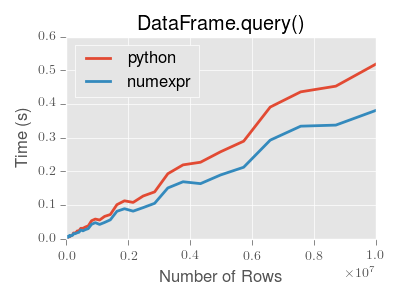
Note
You will only see the performance benefits of using the numexpr engine
with DataFrame.query() if your frame has more than approximately 200,000
rows.
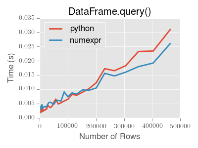
This plot was created using a DataFrame with 3 columns each containing
floating point values generated using numpy.random.randn().
Duplicate Data
If you want to identify and remove duplicate rows in a DataFrame, there are
two methods that will help: duplicated and drop_duplicates. Each
takes as an argument the columns to use to identify duplicated rows.
duplicatedreturns a boolean vector whose length is the number of rows, and which indicates whether a row is duplicated.drop_duplicatesremoves duplicate rows.
By default, the first observed row of a duplicate set is considered unique, but
each method has a keep parameter to specify targets to be kept.
keep='first'(default): mark / drop duplicates except for the first occurrence.keep='last': mark / drop duplicates except for the last occurrence.keep=False: mark / drop all duplicates.
In [268]: df2 = pd.DataFrame({'a': ['one', 'one', 'two', 'two', 'two', 'three', 'four'],
   .....:                     'b': ['x', 'y', 'x', 'y', 'x', 'x', 'x'],
   .....:                     'c': np.random.randn(7)})
   .....:

In [269]: df2
Out[269]:
       a  b         c
0    one  x -1.067137
1    one  y  0.309500
2    two  x -0.211056
3    two  y -1.842023
4    two  x -0.390820
5  three  x -1.964475
6   four  x  1.298329

In [270]: df2.duplicated('a')
Out[270]:
0    False
1     True
2    False
3     True
4     True
5    False
6    False
dtype: bool

In [271]: df2.duplicated('a', keep='last')
Out[271]:
0     True
1    False
2     True
3     True
4    False
5    False
6    False
dtype: bool

In [272]: df2.duplicated('a', keep=False)
Out[272]:
0     True
1     True
2     True
3     True
4     True
5    False
6    False
dtype: bool

In [273]: df2.drop_duplicates('a')
Out[273]:
       a  b         c
0    one  x -1.067137
2    two  x -0.211056
5  three  x -1.964475
6   four  x  1.298329

In [274]: df2.drop_duplicates('a', keep='last')
Out[274]:
       a  b         c
1    one  y  0.309500
4    two  x -0.390820
5  three  x -1.964475
6   four  x  1.298329

In [275]: df2.drop_duplicates('a', keep=False)
Out[275]:
       a  b         c
5  three  x -1.964475
6   four  x  1.298329
Also, you can pass a list of columns to identify duplications.
In [276]: df2.duplicated(['a', 'b'])
Out[276]:
0    False
1    False
2    False
3    False
4     True
5    False
6    False
dtype: bool

In [277]: df2.drop_duplicates(['a', 'b'])
Out[277]:
       a  b         c
0    one  x -1.067137
1    one  y  0.309500
2    two  x -0.211056
3    two  y -1.842023
5  three  x -1.964475
6   four  x  1.298329
To drop duplicates by index value, use Index.duplicated then perform slicing.
The same set of options are available for the keep parameter.
In [278]: df3 = pd.DataFrame({'a': np.arange(6),
   .....:                     'b': np.random.randn(6)},
   .....:                    index=['a', 'a', 'b', 'c', 'b', 'a'])
   .....:

In [279]: df3
Out[279]:
   a         b
a  0  1.440455
a  1  2.456086
b  2  1.038402
c  3 -0.894409
b  4  0.683536
a  5  3.082764

In [280]: df3.index.duplicated()
Out[280]: array([False,  True, False, False,  True,  True], dtype=bool)

In [281]: df3[~df3.index.duplicated()]
Out[281]:
   a         b
a  0  1.440455
b  2  1.038402
c  3 -0.894409

In [282]: df3[~df3.index.duplicated(keep='last')]
Out[282]:
   a         b
c  3 -0.894409
b  4  0.683536
a  5  3.082764

In [283]: df3[~df3.index.duplicated(keep=False)]
Out[283]:
   a         b
c  3 -0.894409
Dictionary-like get() method
Each of Series, DataFrame, and Panel have a get method which can return a
default value.
In [284]: s = pd.Series([1,2,3], index=['a','b','c'])

In [285]: s.get('a')               # equivalent to s['a']
Out[285]: 1

In [286]: s.get('x', default=-1)
Out[286]: -1
The lookup() Method
Sometimes you want to extract a set of values given a sequence of row labels
and column labels, and the lookup method allows for this and returns a
NumPy array. For instance:
In [287]: dflookup = pd.DataFrame(np.random.rand(20,4), columns = ['A','B','C','D'])

In [288]: dflookup.lookup(list(range(0,10,2)), ['B','C','A','B','D'])
Out[288]: array([ 0.3506,  0.4779,  0.4825,  0.9197,  0.5019])
Index objects
The pandas Index class and its subclasses can be viewed as
implementing an ordered multiset. Duplicates are allowed. However, if you try
to convert an Index object with duplicate entries into a
set, an exception will be raised.
Index also provides the infrastructure necessary for
lookups, data alignment, and reindexing. The easiest way to create an
Index directly is to pass a list or other sequence to
Index:
In [289]: index = pd.Index(['e', 'd', 'a', 'b'])

In [290]: index
Out[290]: Index(['e', 'd', 'a', 'b'], dtype='object')

In [291]: 'd' in index
Out[291]: True
You can also pass a name to be stored in the index:
In [292]: index = pd.Index(['e', 'd', 'a', 'b'], name='something')

In [293]: index.name
Out[293]: 'something'
The name, if set, will be shown in the console display:
In [294]: index = pd.Index(list(range(5)), name='rows')

In [295]: columns = pd.Index(['A', 'B', 'C'], name='cols')

In [296]: df = pd.DataFrame(np.random.randn(5, 3), index=index, columns=columns)

In [297]: df
Out[297]:
cols         A         B         C
rows
0     1.295989  0.185778  0.436259
1     0.678101  0.311369 -0.528378
2    -0.674808 -1.103529 -0.656157
3     1.889957  2.076651 -1.102192
4    -1.211795 -0.791746  0.634724

In [298]: df['A']
Out[298]:
rows
0    1.295989
1    0.678101
2   -0.674808
3    1.889957
4   -1.211795
Name: A, dtype: float64
Setting metadata
Indexes are “mostly immutable”, but it is possible to set and change their
metadata, like the index name (or, for MultiIndex, levels and
labels).
You can use the rename, set_names, set_levels, and set_labels
to set these attributes directly. They default to returning a copy; however,
you can specify inplace=True to have the data change in place.
See Advanced Indexing for usage of MultiIndexes.
In [299]: ind = pd.Index([1, 2, 3])

In [300]: ind.rename("apple")
Out[300]: Int64Index([1, 2, 3], dtype='int64', name='apple')

In [301]: ind
Out[301]: Int64Index([1, 2, 3], dtype='int64')

In [302]: ind.set_names(["apple"], inplace=True)

In [303]: ind.name = "bob"

In [304]: ind
Out[304]: Int64Index([1, 2, 3], dtype='int64', name='bob')
set_names, set_levels, and set_labels also take an optional
level` argument
In [305]: index = pd.MultiIndex.from_product([range(3), ['one', 'two']], names=['first', 'second'])

In [306]: index
Out[306]:
MultiIndex(levels=[[0, 1, 2], ['one', 'two']],
           labels=[[0, 0, 1, 1, 2, 2], [0, 1, 0, 1, 0, 1]],
           names=['first', 'second'])

In [307]: index.levels[1]
Out[307]: Index(['one', 'two'], dtype='object', name='second')

In [308]: index.set_levels(["a", "b"], level=1)
Out[308]:
MultiIndex(levels=[[0, 1, 2], ['a', 'b']],
           labels=[[0, 0, 1, 1, 2, 2], [0, 1, 0, 1, 0, 1]],
           names=['first', 'second'])
Set operations on Index objects
The two main operations are union (|) and intersection (&).
These can be directly called as instance methods or used via overloaded
operators. Difference is provided via the .difference() method.
In [309]: a = pd.Index(['c', 'b', 'a'])

In [310]: b = pd.Index(['c', 'e', 'd'])

In [311]: a | b
Out[311]: Index(['a', 'b', 'c', 'd', 'e'], dtype='object')

In [312]: a & b
Out[312]: Index(['c'], dtype='object')

In [313]: a.difference(b)
Out[313]: Index(['a', 'b'], dtype='object')
Also available is the symmetric_difference (^) operation, which returns elements
that appear in either idx1 or idx2, but not in both. This is
equivalent to the Index created by idx1.difference(idx2).union(idx2.difference(idx1)),
with duplicates dropped.
In [314]: idx1 = pd.Index([1, 2, 3, 4])

In [315]: idx2 = pd.Index([2, 3, 4, 5])

In [316]: idx1.symmetric_difference(idx2)
Out[316]: Int64Index([1, 5], dtype='int64')

In [317]: idx1 ^ idx2
Out[317]: Int64Index([1, 5], dtype='int64')
Note
The resulting index from a set operation will be sorted in ascending order.
Missing values
Important
Even though Index can hold missing values (NaN), it should be avoided
if you do not want any unexpected results. For example, some operations
exclude missing values implicitly.
Index.fillna fills missing values with specified scalar value.
In [318]: idx1 = pd.Index([1, np.nan, 3, 4])

In [319]: idx1
Out[319]: Float64Index([1.0, nan, 3.0, 4.0], dtype='float64')

In [320]: idx1.fillna(2)
Out[320]: Float64Index([1.0, 2.0, 3.0, 4.0], dtype='float64')

In [321]: idx2 = pd.DatetimeIndex([pd.Timestamp('2011-01-01'), pd.NaT, pd.Timestamp('2011-01-03')])

In [322]: idx2
Out[322]: DatetimeIndex(['2011-01-01', 'NaT', '2011-01-03'], dtype='datetime64[ns]', freq=None)

In [323]: idx2.fillna(pd.Timestamp('2011-01-02'))
Out[323]: DatetimeIndex(['2011-01-01', '2011-01-02', '2011-01-03'], dtype='datetime64[ns]', freq=None)
Set / Reset Index
Occasionally you will load or create a data set into a DataFrame and want to add an index after you’ve already done so. There are a couple of different ways.
Set an index
DataFrame has a set_index() method which takes a column name
(for a regular Index) or a list of column names (for a MultiIndex).
To create a new, re-indexed DataFrame:
In [324]: data
Out[324]:
     a    b  c    d
0  bar  one  z  1.0
1  bar  two  y  2.0
2  foo  one  x  3.0
3  foo  two  w  4.0

In [325]: indexed1 = data.set_index('c')

In [326]: indexed1
Out[326]:
     a    b    d
c
z  bar  one  1.0
y  bar  two  2.0
x  foo  one  3.0
w  foo  two  4.0

In [327]: indexed2 = data.set_index(['a', 'b'])

In [328]: indexed2
Out[328]:
         c    d
a   b
bar one  z  1.0
    two  y  2.0
foo one  x  3.0
    two  w  4.0
The append keyword option allow you to keep the existing index and append
the given columns to a MultiIndex:
In [329]: frame = data.set_index('c', drop=False)

In [330]: frame = frame.set_index(['a', 'b'], append=True)

In [331]: frame
Out[331]:
           c    d
c a   b
z bar one  z  1.0
y bar two  y  2.0
x foo one  x  3.0
w foo two  w  4.0
Other options in set_index allow you not drop the index columns or to add
the index in-place (without creating a new object):
In [332]: data.set_index('c', drop=False)
Out[332]:
     a    b  c    d
c
z  bar  one  z  1.0
y  bar  two  y  2.0
x  foo  one  x  3.0
w  foo  two  w  4.0

In [333]: data.set_index(['a', 'b'], inplace=True)

In [334]: data
Out[334]:
         c    d
a   b
bar one  z  1.0
    two  y  2.0
foo one  x  3.0
    two  w  4.0
Reset the index
As a convenience, there is a new function on DataFrame called
reset_index() which transfers the index values into the
DataFrame’s columns and sets a simple integer index.
This is the inverse operation of set_index().
In [335]: data
Out[335]:
         c    d
a   b
bar one  z  1.0
    two  y  2.0
foo one  x  3.0
    two  w  4.0

In [336]: data.reset_index()
Out[336]:
     a    b  c    d
0  bar  one  z  1.0
1  bar  two  y  2.0
2  foo  one  x  3.0
3  foo  two  w  4.0
The output is more similar to a SQL table or a record array. The names for the
columns derived from the index are the ones stored in the names attribute.
You can use the level keyword to remove only a portion of the index:
In [337]: frame
Out[337]:
           c    d
c a   b
z bar one  z  1.0
y bar two  y  2.0
x foo one  x  3.0
w foo two  w  4.0

In [338]: frame.reset_index(level=1)
Out[338]:
         a  c    d
c b
z one  bar  z  1.0
y two  bar  y  2.0
x one  foo  x  3.0
w two  foo  w  4.0
reset_index takes an optional parameter drop which if true simply
discards the index, instead of putting index values in the DataFrame’s columns.
Adding an ad hoc index
If you create an index yourself, you can just assign it to the index field:
data.index = index
Returning a view versus a copy
When setting values in a pandas object, care must be taken to avoid what is called
chained indexing. Here is an example.
In [339]: dfmi = pd.DataFrame([list('abcd'),
   .....:                      list('efgh'),
   .....:                      list('ijkl'),
   .....:                      list('mnop')],
   .....:                     columns=pd.MultiIndex.from_product([['one','two'],
   .....:                                                         ['first','second']]))
   .....:

In [340]: dfmi
Out[340]:
    one          two
  first second first second
0     a      b     c      d
1     e      f     g      h
2     i      j     k      l
3     m      n     o      p
Compare these two access methods:
In [341]: dfmi['one']['second']
Out[341]:
0    b
1    f
2    j
3    n
Name: second, dtype: object
In [342]: dfmi.loc[:,('one','second')]
Out[342]:
0    b
1    f
2    j
3    n
Name: (one, second), dtype: object
These both yield the same results, so which should you use? It is instructive to understand the order
of operations on these and why method 2 (.loc) is much preferred over method 1 (chained []).
dfmi['one'] selects the first level of the columns and returns a DataFrame that is singly-indexed.
Then another Python operation dfmi_with_one['second'] selects the series indexed by 'second'.
This is indicated by the variable dfmi_with_one because pandas sees these operations as separate events.
e.g. separate calls to __getitem__, so it has to treat them as linear operations, they happen one after another.
Contrast this to df.loc[:,('one','second')] which passes a nested tuple of (slice(None),('one','second')) to a single call to
__getitem__. This allows pandas to deal with this as a single entity. Furthermore this order of operations can be significantly
faster, and allows one to index both axes if so desired.
Why does assignment fail when using chained indexing?
The problem in the previous section is just a performance issue. What’s up with
the SettingWithCopy warning? We don’t usually throw warnings around when
you do something that might cost a few extra milliseconds!
But it turns out that assigning to the product of chained indexing has inherently unpredictable results. To see this, think about how the Python interpreter executes this code:
dfmi.loc[:,('one','second')] = value
# becomes
dfmi.loc.__setitem__((slice(None), ('one', 'second')), value)
But this code is handled differently:
dfmi['one']['second'] = value
# becomes
dfmi.__getitem__('one').__setitem__('second', value)
See that __getitem__ in there? Outside of simple cases, it’s very hard to
predict whether it will return a view or a copy (it depends on the memory layout
of the array, about which pandas makes no guarantees), and therefore whether
the __setitem__ will modify dfmi or a temporary object that gets thrown
out immediately afterward. That’s what SettingWithCopy is warning you
about!
Note
You may be wondering whether we should be concerned about the loc
property in the first example. But dfmi.loc is guaranteed to be dfmi
itself with modified indexing behavior, so dfmi.loc.__getitem__ /
dfmi.loc.__setitem__ operate on dfmi directly. Of course,
dfmi.loc.__getitem__(idx) may be a view or a copy of dfmi.
Sometimes a SettingWithCopy warning will arise at times when there’s no
obvious chained indexing going on. These are the bugs that
SettingWithCopy is designed to catch! Pandas is probably trying to warn you
that you’ve done this:
def do_something(df):
   foo = df[['bar', 'baz']]  # Is foo a view? A copy? Nobody knows!
   # ... many lines here ...
   foo['quux'] = value       # We don't know whether this will modify df or not!
   return foo
Yikes!
Evaluation order matters
When you use chained indexing, the order and type of the indexing operation partially determine whether the result is a slice into the original object, or a copy of the slice.
Pandas has the SettingWithCopyWarning because assigning to a copy of a
slice is frequently not intentional, but a mistake caused by chained indexing
returning a copy where a slice was expected.
If you would like pandas to be more or less trusting about assignment to a
chained indexing expression, you can set the option
mode.chained_assignment to one of these values:
'warn', the default, means aSettingWithCopyWarningis printed.'raise'means pandas will raise aSettingWithCopyExceptionyou have to deal with.Nonewill suppress the warnings entirely.
In [343]: dfb = pd.DataFrame({'a' : ['one', 'one', 'two',
   .....:                            'three', 'two', 'one', 'six'],
   .....:                     'c' : np.arange(7)})
   .....:

# This will show the SettingWithCopyWarning
# but the frame values will be set
In [344]: dfb['c'][dfb.a.str.startswith('o')] = 42
This however is operating on a copy and will not work.
>>> pd.set_option('mode.chained_assignment','warn')
>>> dfb[dfb.a.str.startswith('o')]['c'] = 42
Traceback (most recent call last)
     ...
SettingWithCopyWarning:
     A value is trying to be set on a copy of a slice from a DataFrame.
     Try using .loc[row_index,col_indexer] = value instead
A chained assignment can also crop up in setting in a mixed dtype frame.
Note
These setting rules apply to all of .loc/.iloc.
This is the correct access method:
In [345]: dfc = pd.DataFrame({'A':['aaa','bbb','ccc'],'B':[1,2,3]})

In [346]: dfc.loc[0,'A'] = 11

In [347]: dfc
Out[347]:
     A  B
0   11  1
1  bbb  2
2  ccc  3
This can work at times, but it is not guaranteed to, and therefore should be avoided:
In [348]: dfc = dfc.copy()

In [349]: dfc['A'][0] = 111

In [350]: dfc
Out[350]:
     A  B
0  111  1
1  bbb  2
2  ccc  3
This will not work at all, and so should be avoided:
>>> pd.set_option('mode.chained_assignment','raise')
>>> dfc.loc[0]['A'] = 1111
Traceback (most recent call last)
     ...
SettingWithCopyException:
     A value is trying to be set on a copy of a slice from a DataFrame.
     Try using .loc[row_index,col_indexer] = value instead
Warning
The chained assignment warnings / exceptions are aiming to inform the user of a possibly invalid assignment. There may be false positives; situations where a chained assignment is inadvertently reported.