使用逻辑回归分类MNIST数字

Note

This sections assumes familiarity with the following Theano concepts: shared variables , basic arithmetic ops , T.grad , floatX. 如果你打算在GPU上运行代码，还要阅读GPU。

Note

The code for this section is available for download here.

在本节中，我们将演示如何使用Theano来实现最基本的分类器：逻辑回归。我们从模型的一个快速入门开始，它既可以作为一个补习，同时也巩固了符号。它演示了数学表达式是如何映射到Theano图上的。

在深度机器学习传统中，本教程将解决MNIST数字分类这个令人激动的问题。

模型

Logistic regression is a probabilistic, linear classifier. 它的参数为一个权重矩阵和一个偏置向量。模型通过将一个输入向量投影到一组超平面上来进行分类，每个超平面对应于一个分类。输入与超平面之间的距离反映了这个输入属于该超平面对应的分类的概率。

在数学上，输入向量属于分类（随机变量的值）的概率可以写为：

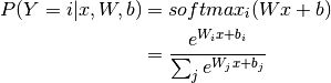
模型的预测结果是概率最大的类，具体为：

The code to do this in Theano is the following:

        # initialize with 0 the weights W as a matrix of shape (n_in, n_out)
        self.W = theano.shared(
            value=numpy.zeros(
                (n_in, n_out),
                dtype=theano.config.floatX
            ),
            name='W',
            borrow=True
        )
        # initialize the biases b as a vector of n_out 0s
        self.b = theano.shared(
            value=numpy.zeros(
                (n_out,),
                dtype=theano.config.floatX
            ),
            name='b',
            borrow=True
        )

        # symbolic expression for computing the matrix of class-membership
        # probabilities
        # Where:
        # W is a matrix where column-k represent the separation hyperplane for
        # class-k
        # x is a matrix where row-j  represents input training sample-j
        # b is a vector where element-k represent the free parameter of
        # hyperplane-k
        self.p_y_given_x = T.nnet.softmax(T.dot(input, self.W) + self.b)

        # symbolic description of how to compute prediction as class whose
        # probability is maximal
        self.y_pred = T.argmax(self.p_y_given_x, axis=1)

由于模型的参数必须在整个训练过程中保持持久状态，因此我们将储存在共享变量中。这表明它们都是符号化的Theano变量，同时也初始化了它们的内容。然后使用了dot和softmax运算符（operator）来计算向量。计算结果p_y_given_x是向量类型的符号变量。

为了获得实际的模型预测结果，我们可以使用T.argmax运算符，它将返回p_y_given_x取最大值时的索引（即，具有最大概率的类）。

显然，我们目前定义的模型还不能起什么作用，因为它的参数仍然是初始化状态。The following section will thus cover how to learn the optimal parameters.

Note

For a complete list of Theano ops, see: list of ops

定义损失函数

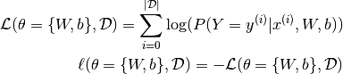
要学习最优模型的参数，就要最小化损失函数。在多分类logistic回归问题中，使用负对数似然函数作为损失函数是非常常见的。这等同于对以为参数的模型最大化其数据集的似然函数。我们首先定义一下似然函数和损失函数：

虽然整本书专注于最小化这个主题，但是梯度下降是迄今为止最小化任意非线性函数的最简单的方法。本教程将使用小批量随机梯度法（MSGD）。See Stochastic Gradient Descent for more details.

以下的Theano代码定义了给定minibatch的（符号化）损失函数：

        # y.shape[0] is (symbolically) the number of rows in y, i.e.,
        # number of examples (call it n) in the minibatch
        # T.arange(y.shape[0]) is a symbolic vector which will contain
        # [0,1,2,... n-1] T.log(self.p_y_given_x) is a matrix of
        # Log-Probabilities (call it LP) with one row per example and
        # one column per class LP[T.arange(y.shape[0]),y] is a vector
        # v containing [LP[0,y[0]], LP[1,y[1]], LP[2,y[2]], ...,
        # LP[n-1,y[n-1]]] and T.mean(LP[T.arange(y.shape[0]),y]) is
        # the mean (across minibatch examples) of the elements in v,
        # i.e., the mean log-likelihood across the minibatch.
        return -T.mean(T.log(self.p_y_given_x)[T.arange(y.shape[0]), y])

Note

虽然损失函数形式上被定义为数据集所有个体误差项的加和sum，但是在实践中，我们在代码中使用的是其平均值（T.mean）。这使得学习速率更少地受minibatch大小的影响。

创建一个LogisticRegression类

We now have all the tools we need to define a LogisticRegression class, which encapsulates the basic behaviour of logistic regression. The code is very similar to what we have covered so far, and should be self explanatory.

class LogisticRegression(object):
    """Multi-class Logistic Regression Class

    The logistic regression is fully described by a weight matrix :math:`W`
    and bias vector :math:`b`. Classification is done by projecting data
    points onto a set of hyperplanes, the distance to which is used to
    determine a class membership probability.
    """

    def __init__(self, input, n_in, n_out):
        """ Initialize the parameters of the logistic regression

        :type input: theano.tensor.TensorType
        :param input: symbolic variable that describes the input of the
                      architecture (one minibatch)

        :type n_in: int
        :param n_in: number of input units, the dimension of the space in
                     which the datapoints lie

        :type n_out: int
        :param n_out: number of output units, the dimension of the space in
                      which the labels lie

        """
        # start-snippet-1
        # initialize with 0 the weights W as a matrix of shape (n_in, n_out)
        self.W = theano.shared(
            value=numpy.zeros(
                (n_in, n_out),
                dtype=theano.config.floatX
            ),
            name='W',
            borrow=True
        )
        # initialize the biases b as a vector of n_out 0s
        self.b = theano.shared(
            value=numpy.zeros(
                (n_out,),
                dtype=theano.config.floatX
            ),
            name='b',
            borrow=True
        )

        # symbolic expression for computing the matrix of class-membership
        # probabilities
        # Where:
        # W is a matrix where column-k represent the separation hyperplane for
        # class-k
        # x is a matrix where row-j  represents input training sample-j
        # b is a vector where element-k represent the free parameter of
        # hyperplane-k
        self.p_y_given_x = T.nnet.softmax(T.dot(input, self.W) + self.b)

        # symbolic description of how to compute prediction as class whose
        # probability is maximal
        self.y_pred = T.argmax(self.p_y_given_x, axis=1)
        # end-snippet-1

        # parameters of the model
        self.params = [self.W, self.b]

        # keep track of model input
        self.input = input

    def negative_log_likelihood(self, y):
        """Return the mean of the negative log-likelihood of the prediction
        of this model under a given target distribution.

        .. math::

            \frac{1}{|\mathcal{D}|} \mathcal{L} (\theta=\{W,b\}, \mathcal{D}) =
            \frac{1}{|\mathcal{D}|} \sum_{i=0}^{|\mathcal{D}|}
                \log(P(Y=y^{(i)}|x^{(i)}, W,b)) \\
            \ell (\theta=\{W,b\}, \mathcal{D})

        :type y: theano.tensor.TensorType
        :param y: corresponds to a vector that gives for each example the
                  correct label

        Note: we use the mean instead of the sum so that
              the learning rate is less dependent on the batch size
        """
        # start-snippet-2
        # y.shape[0] is (symbolically) the number of rows in y, i.e.,
        # number of examples (call it n) in the minibatch
        # T.arange(y.shape[0]) is a symbolic vector which will contain
        # [0,1,2,... n-1] T.log(self.p_y_given_x) is a matrix of
        # Log-Probabilities (call it LP) with one row per example and
        # one column per class LP[T.arange(y.shape[0]),y] is a vector
        # v containing [LP[0,y[0]], LP[1,y[1]], LP[2,y[2]], ...,
        # LP[n-1,y[n-1]]] and T.mean(LP[T.arange(y.shape[0]),y]) is
        # the mean (across minibatch examples) of the elements in v,
        # i.e., the mean log-likelihood across the minibatch.
        return -T.mean(T.log(self.p_y_given_x)[T.arange(y.shape[0]), y])
        # end-snippet-2

    def errors(self, y):
        """Return a float representing the number of errors in the minibatch
        over the total number of examples of the minibatch ; zero one
        loss over the size of the minibatch

        :type y: theano.tensor.TensorType
        :param y: corresponds to a vector that gives for each example the
                  correct label
        """

        # check if y has same dimension of y_pred
        if y.ndim != self.y_pred.ndim:
            raise TypeError(
                'y should have the same shape as self.y_pred',
                ('y', y.type, 'y_pred', self.y_pred.type)
            )
        # check if y is of the correct datatype
        if y.dtype.startswith('int'):
            # the T.neq operator returns a vector of 0s and 1s, where 1
            # represents a mistake in prediction
            return T.mean(T.neq(self.y_pred, y))
        else:
            raise NotImplementedError()

我们定义一个这个类的实例，如下所示：

    # generate symbolic variables for input (x and y represent a
    # minibatch)
    x = T.matrix('x')  # data, presented as rasterized images
    y = T.ivector('y')  # labels, presented as 1D vector of [int] labels

    # construct the logistic regression class
    # Each MNIST image has size 28*28
    classifier = LogisticRegression(input=x, n_in=28 * 28, n_out=10)

We start by allocating symbolic variables for the training inputs and their corresponding classes . 请注意，x和y定义在LogisticRegression对象的作用域之外。Since the class requires the input to build its graph, it is passed as a parameter of the __init__ function. This is useful in case you want to connect instances of such classes to form a deep network. 一层网络的输出可作为上层网络的输入而传递。(This tutorial does not build a multi-layer network, but this code will be reused in future tutorials that do.)

Finally, we define a (symbolic) cost variable to minimize, using the instance method classifier.negative_log_likelihood.

    # the cost we minimize during training is the negative log likelihood of
    # the model in symbolic format
    cost = classifier.negative_log_likelihood(y)

注意，x是cost定义的隐式符号输入，因为classifier的符号变量在初始化时以x定义。

学习模型

为了在大多数编程语言（C/C++、Matlab、Python）中实现MSGD，可以手动导出损失函数关于参数的梯度的表达式：在这个例子中为和，对于复杂的模型，这可能会很棘手，因为的表达式可能会变得相当复杂，尤其是要考虑数值稳定性的问题时。

利用Theano，这项工作被大大简化。It performs automatic differentiation and applies certain math transforms to improve numerical stability.

在Theano中，要得到梯度和，只需执行以下操作：

    g_W = T.grad(cost=cost, wrt=classifier.W)
    g_b = T.grad(cost=cost, wrt=classifier.b)

g_W and g_b are symbolic variables, which can be used as part of a computation graph. 单次执行梯度下降的函数train_model可以定义如下：

    # specify how to update the parameters of the model as a list of
    # (variable, update expression) pairs.
    updates = [(classifier.W, classifier.W - learning_rate * g_W),
               (classifier.b, classifier.b - learning_rate * g_b)]

    # compiling a Theano function `train_model` that returns the cost, but in
    # the same time updates the parameter of the model based on the rules
    # defined in `updates`
    train_model = theano.function(
        inputs=[index],
        outputs=cost,
        updates=updates,
        givens={
            x: train_set_x[index * batch_size: (index + 1) * batch_size],
            y: train_set_y[index * batch_size: (index + 1) * batch_size]
        }
    )

updates是一个元素为配对的列表。在每个配对中，第一个元素是在该步骤中要更新的符号变量，第二个元素是用于计算其新值的符号函数。类似地，givens是一个字典，其键是符号变量，键值在该步骤中指定它们的替换值。The function train_model is then defined such that:

• 输入是mini-batch的索引index，其与batch的大小（它不是输入，因为它是固定的）一起定义具有相应标签的
• 返回值是与由index所定义的x、y相关联的cost/loss（损失）函数
• 每次调用函数时，它会先用由index指定的训练集的切片来更新x和y。然后，它会计算与该minibatch相对应的损失函数，再实施由updates列表所定义的操作。

每次调用train_model(index)时，它将计算并返回minibatch的cost，同时执行一次MSGD。因此，循环遍历数据集中的所有样本，一次只考虑一个minibatch中的所有样本，并重复调用train_model函数，这样便组成了整个学习算法。

测试模型

如Learning a Classifier中所述，在测试模型时，我们会对被错误分类的样本的数量感兴趣（而不仅仅是似然函数）。因此，LogisticRegression类具有一个额外的实例方法，它构建了符号图用于获取每个minibatch中的错误分类样本的数量。

The code is as follows:

    def errors(self, y):
        """Return a float representing the number of errors in the minibatch
        over the total number of examples of the minibatch ; zero one
        loss over the size of the minibatch

        :type y: theano.tensor.TensorType
        :param y: corresponds to a vector that gives for each example the
                  correct label
        """

        # check if y has same dimension of y_pred
        if y.ndim != self.y_pred.ndim:
            raise TypeError(
                'y should have the same shape as self.y_pred',
                ('y', y.type, 'y_pred', self.y_pred.type)
            )
        # check if y is of the correct datatype
        if y.dtype.startswith('int'):
            # the T.neq operator returns a vector of 0s and 1s, where 1
            # represents a mistake in prediction
            return T.mean(T.neq(self.y_pred, y))
        else:
            raise NotImplementedError()

然后，我们创建一个test_model函数和一个validate_model函数，我们可以调用它们来获取这个值。正如你将看到的，validate_model是我们实施提前停止的关键（参见提前停止）。这些函数接受一个minibatch索引，并为该minibatch中的样本计算模型错误分类的数目。它们之间的唯一区别是test_model从测试集中抽取minibatches，而validate_model从验证集中抽取。

    # compiling a Theano function that computes the mistakes that are made by
    # the model on a minibatch
    test_model = theano.function(
        inputs=[index],
        outputs=classifier.errors(y),
        givens={
            x: test_set_x[index * batch_size: (index + 1) * batch_size],
            y: test_set_y[index * batch_size: (index + 1) * batch_size]
        }
    )

    validate_model = theano.function(
        inputs=[index],
        outputs=classifier.errors(y),
        givens={
            x: valid_set_x[index * batch_size: (index + 1) * batch_size],
            y: valid_set_y[index * batch_size: (index + 1) * batch_size]
        }
    )

合在一起

The finished product is as follows.

"""
This tutorial introduces logistic regression using Theano and stochastic
gradient descent.

Logistic regression is a probabilistic, linear classifier. It is parametrized
by a weight matrix :math:`W` and a bias vector :math:`b`. Classification is
done by projecting data points onto a set of hyperplanes, the distance to
which is used to determine a class membership probability.

Mathematically, this can be written as:

.. math::
  P(Y=i|x, W,b) &= softmax_i(W x + b) \\
                &= \frac {e^{W_i x + b_i}} {\sum_j e^{W_j x + b_j}}


The output of the model or prediction is then done by taking the argmax of
the vector whose i'th element is P(Y=i|x).

.. math::

  y_{pred} = argmax_i P(Y=i|x,W,b)


This tutorial presents a stochastic gradient descent optimization method
suitable for large datasets.


References:

    - textbooks: "Pattern Recognition and Machine Learning" -
                 Christopher M. Bishop, section 4.3.2

"""

from __future__ import print_function

__docformat__ = 'restructedtext en'

import six.moves.cPickle as pickle
import gzip
import os
import sys
import timeit

import numpy

import theano
import theano.tensor as T


class LogisticRegression(object):
    """Multi-class Logistic Regression Class

    The logistic regression is fully described by a weight matrix :math:`W`
    and bias vector :math:`b`. Classification is done by projecting data
    points onto a set of hyperplanes, the distance to which is used to
    determine a class membership probability.
    """

    def __init__(self, input, n_in, n_out):
        """ Initialize the parameters of the logistic regression

        :type input: theano.tensor.TensorType
        :param input: symbolic variable that describes the input of the
                      architecture (one minibatch)

        :type n_in: int
        :param n_in: number of input units, the dimension of the space in
                     which the datapoints lie

        :type n_out: int
        :param n_out: number of output units, the dimension of the space in
                      which the labels lie

        """
        # start-snippet-1
        # initialize with 0 the weights W as a matrix of shape (n_in, n_out)
        self.W = theano.shared(
            value=numpy.zeros(
                (n_in, n_out),
                dtype=theano.config.floatX
            ),
            name='W',
            borrow=True
        )
        # initialize the biases b as a vector of n_out 0s
        self.b = theano.shared(
            value=numpy.zeros(
                (n_out,),
                dtype=theano.config.floatX
            ),
            name='b',
            borrow=True
        )

        # symbolic expression for computing the matrix of class-membership
        # probabilities
        # Where:
        # W is a matrix where column-k represent the separation hyperplane for
        # class-k
        # x is a matrix where row-j  represents input training sample-j
        # b is a vector where element-k represent the free parameter of
        # hyperplane-k
        self.p_y_given_x = T.nnet.softmax(T.dot(input, self.W) + self.b)

        # symbolic description of how to compute prediction as class whose
        # probability is maximal
        self.y_pred = T.argmax(self.p_y_given_x, axis=1)
        # end-snippet-1

        # parameters of the model
        self.params = [self.W, self.b]

        # keep track of model input
        self.input = input

    def negative_log_likelihood(self, y):
        """Return the mean of the negative log-likelihood of the prediction
        of this model under a given target distribution.

        .. math::

            \frac{1}{|\mathcal{D}|} \mathcal{L} (\theta=\{W,b\}, \mathcal{D}) =
            \frac{1}{|\mathcal{D}|} \sum_{i=0}^{|\mathcal{D}|}
                \log(P(Y=y^{(i)}|x^{(i)}, W,b)) \\
            \ell (\theta=\{W,b\}, \mathcal{D})

        :type y: theano.tensor.TensorType
        :param y: corresponds to a vector that gives for each example the
                  correct label

        Note: we use the mean instead of the sum so that
              the learning rate is less dependent on the batch size
        """
        # start-snippet-2
        # y.shape[0] is (symbolically) the number of rows in y, i.e.,
        # number of examples (call it n) in the minibatch
        # T.arange(y.shape[0]) is a symbolic vector which will contain
        # [0,1,2,... n-1] T.log(self.p_y_given_x) is a matrix of
        # Log-Probabilities (call it LP) with one row per example and
        # one column per class LP[T.arange(y.shape[0]),y] is a vector
        # v containing [LP[0,y[0]], LP[1,y[1]], LP[2,y[2]], ...,
        # LP[n-1,y[n-1]]] and T.mean(LP[T.arange(y.shape[0]),y]) is
        # the mean (across minibatch examples) of the elements in v,
        # i.e., the mean log-likelihood across the minibatch.
        return -T.mean(T.log(self.p_y_given_x)[T.arange(y.shape[0]), y])
        # end-snippet-2

    def errors(self, y):
        """Return a float representing the number of errors in the minibatch
        over the total number of examples of the minibatch ; zero one
        loss over the size of the minibatch

        :type y: theano.tensor.TensorType
        :param y: corresponds to a vector that gives for each example the
                  correct label
        """

        # check if y has same dimension of y_pred
        if y.ndim != self.y_pred.ndim:
            raise TypeError(
                'y should have the same shape as self.y_pred',
                ('y', y.type, 'y_pred', self.y_pred.type)
            )
        # check if y is of the correct datatype
        if y.dtype.startswith('int'):
            # the T.neq operator returns a vector of 0s and 1s, where 1
            # represents a mistake in prediction
            return T.mean(T.neq(self.y_pred, y))
        else:
            raise NotImplementedError()


def load_data(dataset):
    ''' Loads the dataset

    :type dataset: string
    :param dataset: the path to the dataset (here MNIST)
    '''

    #############
    # LOAD DATA #
    #############

    # Download the MNIST dataset if it is not present
    data_dir, data_file = os.path.split(dataset)
    if data_dir == "" and not os.path.isfile(dataset):
        # Check if dataset is in the data directory.
        new_path = os.path.join(
            os.path.split(__file__)[0],
            "..",
            "data",
            dataset
        )
        if os.path.isfile(new_path) or data_file == 'mnist.pkl.gz':
            dataset = new_path

    if (not os.path.isfile(dataset)) and data_file == 'mnist.pkl.gz':
        from six.moves import urllib
        origin = (
            'http://www.iro.umontreal.ca/~lisa/deep/data/mnist/mnist.pkl.gz'
        )
        print('Downloading data from %s' % origin)
        urllib.request.urlretrieve(origin, dataset)

    print('... loading data')

    # Load the dataset
    with gzip.open(dataset, 'rb') as f:
        try:
            train_set, valid_set, test_set = pickle.load(f, encoding='latin1')
        except:
            train_set, valid_set, test_set = pickle.load(f)
    # train_set, valid_set, test_set format: tuple(input, target)
    # input is a numpy.ndarray of 2 dimensions (a matrix)
    # where each row corresponds to an example. target is a
    # numpy.ndarray of 1 dimension (vector) that has the same length as
    # the number of rows in the input. It should give the target
    # to the example with the same index in the input.

    def shared_dataset(data_xy, borrow=True):
        """ Function that loads the dataset into shared variables

        The reason we store our dataset in shared variables is to allow
        Theano to copy it into the GPU memory (when code is run on GPU).
        Since copying data into the GPU is slow, copying a minibatch everytime
        is needed (the default behaviour if the data is not in a shared
        variable) would lead to a large decrease in performance.
        """
        data_x, data_y = data_xy
        shared_x = theano.shared(numpy.asarray(data_x,
                                               dtype=theano.config.floatX),
                                 borrow=borrow)
        shared_y = theano.shared(numpy.asarray(data_y,
                                               dtype=theano.config.floatX),
                                 borrow=borrow)
        # When storing data on the GPU it has to be stored as floats
        # therefore we will store the labels as ``floatX`` as well
        # (``shared_y`` does exactly that). But during our computations
        # we need them as ints (we use labels as index, and if they are
        # floats it doesn't make sense) therefore instead of returning
        # ``shared_y`` we will have to cast it to int. This little hack
        # lets ous get around this issue
        return shared_x, T.cast(shared_y, 'int32')

    test_set_x, test_set_y = shared_dataset(test_set)
    valid_set_x, valid_set_y = shared_dataset(valid_set)
    train_set_x, train_set_y = shared_dataset(train_set)

    rval = [(train_set_x, train_set_y), (valid_set_x, valid_set_y),
            (test_set_x, test_set_y)]
    return rval


def sgd_optimization_mnist(learning_rate=0.13, n_epochs=1000,
                           dataset='mnist.pkl.gz',
                           batch_size=600):
    """
    Demonstrate stochastic gradient descent optimization of a log-linear
    model

    This is demonstrated on MNIST.

    :type learning_rate: float
    :param learning_rate: learning rate used (factor for the stochastic
                          gradient)

    :type n_epochs: int
    :param n_epochs: maximal number of epochs to run the optimizer

    :type dataset: string
    :param dataset: the path of the MNIST dataset file from
                 http://www.iro.umontreal.ca/~lisa/deep/data/mnist/mnist.pkl.gz

    """
    datasets = load_data(dataset)

    train_set_x, train_set_y = datasets[0]
    valid_set_x, valid_set_y = datasets[1]
    test_set_x, test_set_y = datasets[2]

    # compute number of minibatches for training, validation and testing
    n_train_batches = train_set_x.get_value(borrow=True).shape[0] // batch_size
    n_valid_batches = valid_set_x.get_value(borrow=True).shape[0] // batch_size
    n_test_batches = test_set_x.get_value(borrow=True).shape[0] // batch_size

    ######################
    # BUILD ACTUAL MODEL #
    ######################
    print('... building the model')

    # allocate symbolic variables for the data
    index = T.lscalar()  # index to a [mini]batch

    # generate symbolic variables for input (x and y represent a
    # minibatch)
    x = T.matrix('x')  # data, presented as rasterized images
    y = T.ivector('y')  # labels, presented as 1D vector of [int] labels

    # construct the logistic regression class
    # Each MNIST image has size 28*28
    classifier = LogisticRegression(input=x, n_in=28 * 28, n_out=10)

    # the cost we minimize during training is the negative log likelihood of
    # the model in symbolic format
    cost = classifier.negative_log_likelihood(y)

    # compiling a Theano function that computes the mistakes that are made by
    # the model on a minibatch
    test_model = theano.function(
        inputs=[index],
        outputs=classifier.errors(y),
        givens={
            x: test_set_x[index * batch_size: (index + 1) * batch_size],
            y: test_set_y[index * batch_size: (index + 1) * batch_size]
        }
    )

    validate_model = theano.function(
        inputs=[index],
        outputs=classifier.errors(y),
        givens={
            x: valid_set_x[index * batch_size: (index + 1) * batch_size],
            y: valid_set_y[index * batch_size: (index + 1) * batch_size]
        }
    )

    # compute the gradient of cost with respect to theta = (W,b)
    g_W = T.grad(cost=cost, wrt=classifier.W)
    g_b = T.grad(cost=cost, wrt=classifier.b)

    # start-snippet-3
    # specify how to update the parameters of the model as a list of
    # (variable, update expression) pairs.
    updates = [(classifier.W, classifier.W - learning_rate * g_W),
               (classifier.b, classifier.b - learning_rate * g_b)]

    # compiling a Theano function `train_model` that returns the cost, but in
    # the same time updates the parameter of the model based on the rules
    # defined in `updates`
    train_model = theano.function(
        inputs=[index],
        outputs=cost,
        updates=updates,
        givens={
            x: train_set_x[index * batch_size: (index + 1) * batch_size],
            y: train_set_y[index * batch_size: (index + 1) * batch_size]
        }
    )
    # end-snippet-3

    ###############
    # TRAIN MODEL #
    ###############
    print('... training the model')
    # early-stopping parameters
    patience = 5000  # look as this many examples regardless
    patience_increase = 2  # wait this much longer when a new best is
                                  # found
    improvement_threshold = 0.995  # a relative improvement of this much is
                                  # considered significant
    validation_frequency = min(n_train_batches, patience // 2)
                                  # go through this many
                                  # minibatche before checking the network
                                  # on the validation set; in this case we
                                  # check every epoch

    best_validation_loss = numpy.inf
    test_score = 0.
    start_time = timeit.default_timer()

    done_looping = False
    epoch = 0
    while (epoch < n_epochs) and (not done_looping):
        epoch = epoch + 1
        for minibatch_index in range(n_train_batches):

            minibatch_avg_cost = train_model(minibatch_index)
            # iteration number
            iter = (epoch - 1) * n_train_batches + minibatch_index

            if (iter + 1) % validation_frequency == 0:
                # compute zero-one loss on validation set
                validation_losses = [validate_model(i)
                                     for i in range(n_valid_batches)]
                this_validation_loss = numpy.mean(validation_losses)

                print(
                    'epoch %i, minibatch %i/%i, validation error %f %%' %
                    (
                        epoch,
                        minibatch_index + 1,
                        n_train_batches,
                        this_validation_loss * 100.
                    )
                )

                # if we got the best validation score until now
                if this_validation_loss < best_validation_loss:
                    #improve patience if loss improvement is good enough
                    if this_validation_loss < best_validation_loss *  \
                       improvement_threshold:
                        patience = max(patience, iter * patience_increase)

                    best_validation_loss = this_validation_loss
                    # test it on the test set

                    test_losses = [test_model(i)
                                   for i in range(n_test_batches)]
                    test_score = numpy.mean(test_losses)

                    print(
                        (
                            '     epoch %i, minibatch %i/%i, test error of'
                            ' best model %f %%'
                        ) %
                        (
                            epoch,
                            minibatch_index + 1,
                            n_train_batches,
                            test_score * 100.
                        )
                    )

                    # save the best model
                    with open('best_model.pkl', 'wb') as f:
                        pickle.dump(classifier, f)

            if patience <= iter:
                done_looping = True
                break

    end_time = timeit.default_timer()
    print(
        (
            'Optimization complete with best validation score of %f %%,'
            'with test performance %f %%'
        )
        % (best_validation_loss * 100., test_score * 100.)
    )
    print('The code run for %d epochs, with %f epochs/sec' % (
        epoch, 1. * epoch / (end_time - start_time)))
    print(('The code for file ' +
           os.path.split(__file__)[1] +
           ' ran for %.1fs' % ((end_time - start_time))), file=sys.stderr)


def predict():
    """
    An example of how to load a trained model and use it
    to predict labels.
    """

    # load the saved model
    classifier = pickle.load(open('best_model.pkl'))

    # compile a predictor function
    predict_model = theano.function(
        inputs=[classifier.input],
        outputs=classifier.y_pred)

    # We can test it on some examples from test test
    dataset='mnist.pkl.gz'
    datasets = load_data(dataset)
    test_set_x, test_set_y = datasets[2]
    test_set_x = test_set_x.get_value()

    predicted_values = predict_model(test_set_x[:10])
    print("Predicted values for the first 10 examples in test set:")
    print(predicted_values)


if __name__ == '__main__':
    sgd_optimization_mnist()

用户可以通过在DeepLearningTutorials文件夹中键入以下语句来学习如何使用SGD逻辑回归分类MNIST数字：

python code/logistic_sgd.py

The output one should expect is of the form :

...
epoch 72, minibatch 83/83, validation error 7.510417 %
     epoch 72, minibatch 83/83, test error of best model 7.510417 %
epoch 73, minibatch 83/83, validation error 7.500000 %
     epoch 73, minibatch 83/83, test error of best model 7.489583 %
Optimization complete with best validation score of 7.500000 %,with test performance 7.489583 %
The code run for 74 epochs, with 1.936983 epochs/sec

在Intel(R) Core(TM)2 Duo CPU E8400 @ 3.00 Ghz上，代码以接近1.936 epochs/s的速度运行，并且运行了75个epochs后得到7.489％的测试误差。在GPU上，代码几乎以10.0 epochs/sec的速度运行。在这个实例中，我们使用的batch大小为600。

使用训练好的模型进行预测

sgd_optimization_mnist serialize and pickle the model each time new lowest validation error is reached. We can reload this model and predict labels of new data. predict function shows an example of how this could be done.

def predict():
    """
    An example of how to load a trained model and use it
    to predict labels.
    """

    # load the saved model
    classifier = pickle.load(open('best_model.pkl'))

    # compile a predictor function
    predict_model = theano.function(
        inputs=[classifier.input],
        outputs=classifier.y_pred)

    # We can test it on some examples from test test
    dataset='mnist.pkl.gz'
    datasets = load_data(dataset)
    test_set_x, test_set_y = datasets[2]
    test_set_x = test_set_x.get_value()

    predicted_values = predict_model(test_set_x[:10])
    print("Predicted values for the first 10 examples in test set:")
    print(predicted_values)

Footnotes

[1]	对于更小的数据集和更简单的模型，有更有效但更复杂的下降算法。The sample code logistic_cg.py demonstrates how to use SciPy’s conjugate gradient solver with Theano on the logistic regression task.