
1.3.5. 一些练习
1.3.5.1. 数组操作
生成一个2-D数组(无需明确输入):
[[1,  6, 11],
 [2,  7, 12],
 [3,  8, 13],
 [4,  9, 14],
 [5, 10, 15]]
and generate a new array containing its 2nd and 4th rows.
将下面数组的每一列:
>>> import numpy as np
>>> a = np.arange(25).reshape(5, 5)
按元素级别除以数组
b = np.array([1. , 5, 10, 15, 20])。(Hint:np.newaxis).更难的:生成一个10 x 3的随机数数组(范围[0,1])。For each row, pick the number closest to 0.5.
- Use
absandargsortto find the columnjclosest for each row. - 使用花式索引来提取数字。(Hint:
a[i,j]– the arrayimust contain the row numbers corresponding to stuff inj.)
- Use
1.3.5.2. 图片处理:框出一张脸
让我们从一个浣熊的图像开始对numpy数组进行一些操作。scipy provides a 2D array of this image with the scipy.misc.face function:
>>> from scipy import misc
>>> face = misc.face(gray=True)  # 2D grayscale image
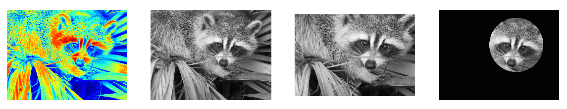
这里有一些图像,我们将能够通过我们的操作获得它们:使用不同的颜色映射,裁剪图像,更改图像的一些部分。
Let’s use the imshow function of pylab to display the image.
>>> import pylab as plt
>>> face = misc.face(gray=True)
>>> plt.imshow(face)
<matplotlib.image.AxesImage object at 0x...>
-
脸部以显示的颜色不对。必须指定色彩映射才能以灰色显示。
>>> plt.imshow(face, cmap=plt.cm.gray)
<matplotlib.image.AxesImage object at 0x...>
-
创建一个具有较窄中心的图像数组,例如从图像的所有边中删除100个像素。To check the result, display this new array with
imshow.>>> crop_face = face[100:-100, 100:-100]
-
We will now frame the face with a black locket. 为此,我们需要创建一个对应于我们想要的黑色像素的掩码。面部的中心在(660, 330)左右,因此我们通过这个条件
(y-300)**2 + (x-660)**2定义掩码>>> sy, sx = face.shape >>> y, x = np.ogrid[0:sy, 0:sx] # x and y indices of pixels >>> y.shape, x.shape ((768, 1), (1, 1024)) >>> centerx, centery = (660, 300) # center of the image >>> mask = ((y - centery)**2 + (x - centerx)**2) > 230**2 # circle
然后,我们将值0赋值给与掩码对应的图像像素。The syntax is extremely simple and intuitive:
>>> face[mask] = 0
>>> plt.imshow(face)
<matplotlib.image.AxesImage object at 0x...>
-
后续:复制本练习的所有指令到一个叫做
face_locket.py的脚本中,然后使用%run face_locket.py在IPython中执行这个脚本。Change the circle to an ellipsoid.
1.3.5.3. 数据统计
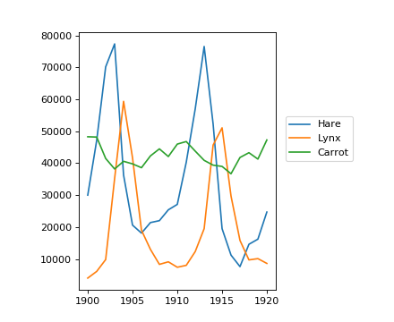
populations.txt中的数据描述了加拿大北部20年期间野兔和(和胡萝卜)的数量:
>>> data = np.loadtxt('data/populations.txt')
>>> year, hares, lynxes, carrots = data.T  # trick: columns to variables

>>> import matplotlib.pyplot as plt
>>> plt.axes([0.2, 0.1, 0.5, 0.8])
<matplotlib.axes...Axes object at ...>
>>> plt.plot(year, hares, year, lynxes, year, carrots)
[<matplotlib.lines.Line2D object at ...>, ...]
>>> plt.legend(('Hare', 'Lynx', 'Carrot'), loc=(1.05, 0.5))
<matplotlib.legend.Legend object at ...>
[source code, hires.png, pdf]
基于populations.txt中的数据计算和打印...
- 期间这些年各个物种数量的平均值和标准差。
- 每个物种在哪一年的数量最多。
- 每年哪个物种的数量最大。(提示:
argsort和花式索引np.array(['H', 'L', 'C'])) - 哪些年份有任何一个物种的数量在50000以上。(Hint: comparisons and
np.any) - 当hare种群数量最少时,每个物种的前2年。(提示:
argsort、花式索引) - 比较(画出)野兔数量的变化(见
help(np.gradient))和胡萝卜数量。Check correlation (seehelp(np.corrcoef)).
...所有的都不需要for循环。
答案:Python源文件
1.3.5.4. 积分的粗略近似
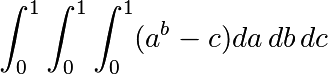
编写一个函数f(a, b, c),返回 。生成一个24x12x6数组,它的值位于参数范围
[0,1] x [0,1] x [0,1]中。
Approximate the 3-d integral
的体积,用平均值。精确的的结果是: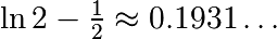 — what is your relative error?
(提示:使用元素级别的操作和broadcasting。你可以使用np.ogrid[0:1:20j]让np.ogrid给出给定范围内一定数目的点数。)
Reminder Python functions:
def f(a, b, c):
    return some_result
答案:Python源文件
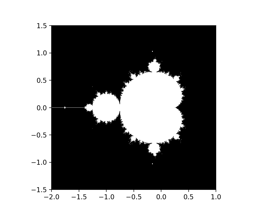
1.3.5.5. Mandelbrot集合
[source code, hires.png, pdf]
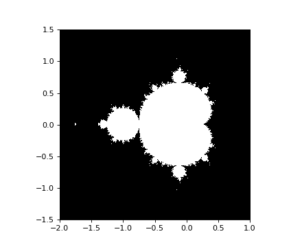
Write a script that computes the Mandelbrot fractal. The Mandelbrot iteration:
N_max = 50
some_threshold = 50

c = x + 1j*y

z = 0
for j in range(N_max):
    z = z**2 + c
点(x, y)属于Mandelbrot集合,如果 <
< some_threshold。
Do this computation by:
- 构造[-2, 1] x [-1.5, 1.5]范围内的c = x + 1j*y值的网格
- Do the iteration
- Form the 2-d boolean mask indicating which points are in the set
- 使用以下语句将结果保存到图像:
>>> import matplotlib.pyplot as plt
>>> plt.imshow(mask.T, extent=[-2, 1, -1.5, 1.5])
<matplotlib.image.AxesImage object at ...>
>>> plt.gray()
>>> plt.savefig('mandelbrot.png')
答案:Python源文件
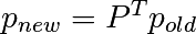
1.3.5.6. 马尔科夫链

Markov chain transition matrix P, and probability distribution on the states p:
0 <= P[i,j] <= 1: 从状态i到状态j的概率- 转移规则:
all(sum(P, axis=1) == 1),p.sum() == 1:规范化
编写一个具有5个状态的脚本,并且:
- 构造一个随机矩阵,并规范化每一行,使其成为一个转移矩阵。
- 从随机(归一化)概率分布
p开始并且需要50步 =>p_50 - 计算状态的分布:具有特征值1(数值:最接近1)的
P.T的特征向量 =>p_stationary
记住归一化特征向量 —— 我没有...
- Checks if
p_50andp_stationaryare equal to tolerance 1e-5
工具:np.random.rand、.dot()、np.linalg.eig、规约、abs()、argmin、比较、all、np.linalg.norm等。
答案:Python源文件