3D Gridded Data

The following section describes the available style settings for 3D-Gridded data objects.

To access the style settings, right-click on the surface data object in the Data Explorer, and select Settings... from the pop-up menu. Then, in the Settings dialog, expand the Style node to view the style settings.

Cells

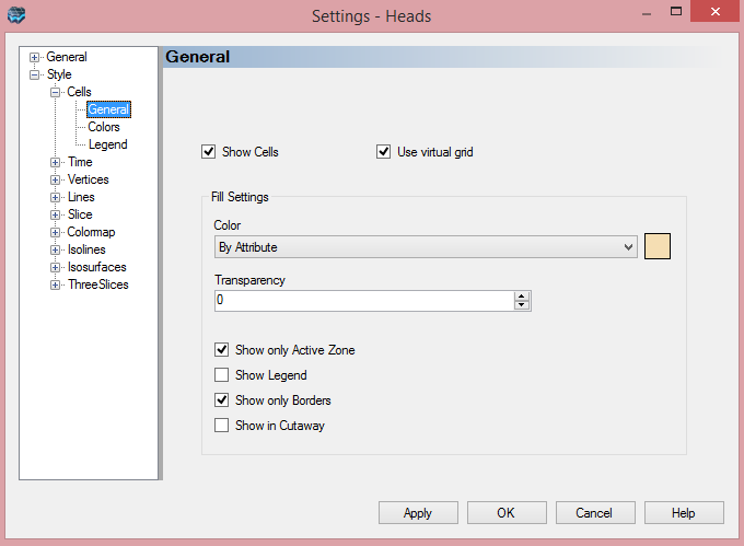
The Cells node allows you to specify style settings for the grid cells. The following options are available:

The Show Cell check box allows you to show/hide the grid cells in the 3D gridded data object. When the check box is selected, you can choose how to show the cells in the Color combo box in the Fill Settings frame. With the Specified option, select the adjacent color swatch and select the desired color to fill the cells. If you select Color by Attribute, you can color each cell according to a specified attribute, e.g., heads. Color by attribute settings can be defined by selecting the Color node, located under the Cells node.

For more information on the color by attribute feature, please refer to "Color By Attribute" section.

The Show only Active Zone check box allows you to show/hide inactive grid cells.

Vertices, Lines

For information on the settings available in the Vertices and Lines nodes, please refer the Points \ Vertices and Lines respectively.

Slice

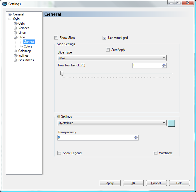
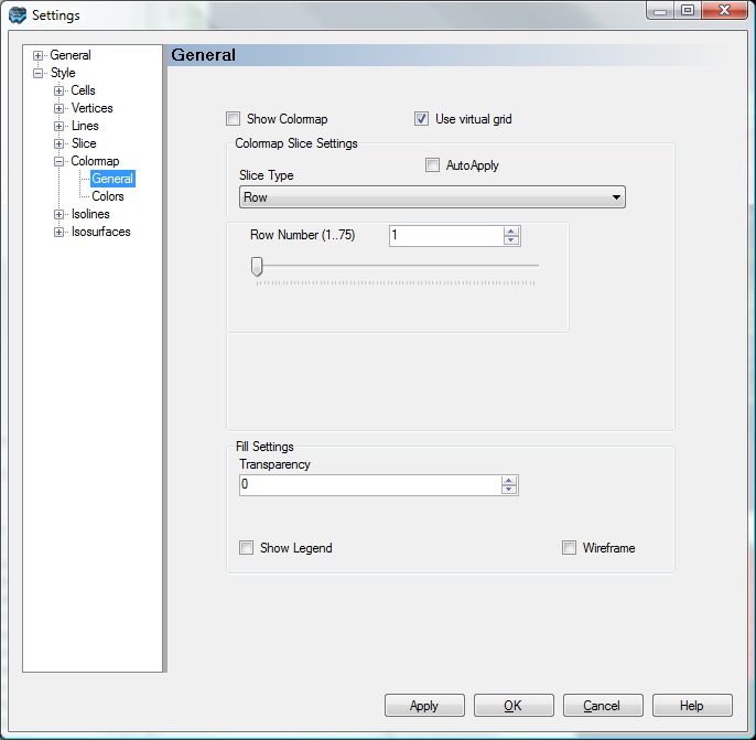
Show Slice will control the display status in the 3D Viewer.

Use Virtual Grid option allows you to use a coarsened version of the true 3d grid dimensions. This option is recommended when you have moderate to large size grids (exceeding a few hundred thousand cells). If you have a small grid then this option can be turned off. For more details, see Virtual Grid Settings

Under Slice Settings, specify the desired Layer, Row, or Column Number.

Under Fill Settings, the ByAttribute option is default and recommended for most cases.

Show Legend check box at the bottom of the window will add a color legend to the current 3d view

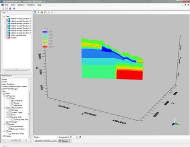
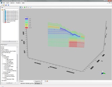
Show Wireframe will render with wireframe instead of filled in cells. The example below illustrates this:

Filled Slice	Wireframe

In the Settings tree, under Slice -- Colors, you can access the color page where you can choose which attribute you want to render; in the case of Properties (or Recharge and Evapotranspiration) you can render by Zone or by the specified Attribute (eg. Kx, Recharge rate, etc..)For more information on the color by attribute feature, please refer to "Color By Attribute" section.

Colormap

Settings for the Colormap are identical to those explained above for Slice.

Plot Color Map on Cross-Sections

Color map has an additional Slice Type, which is "Cross Section" which is shown below:

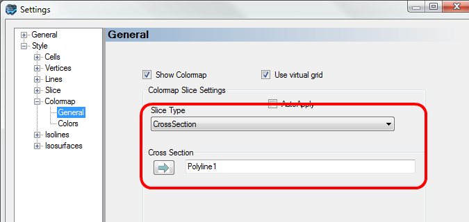
After selecting this Slice Type, you need to provide a polyline data object that contains one or more polylines representing the cross-sections you want to render. Polylines can be imported from a shapefile or DXF file, or created manually. See Creating New Data Objects for more details.

Select this polyline data object from the tree, then click on the to insert this into the field as shown above.

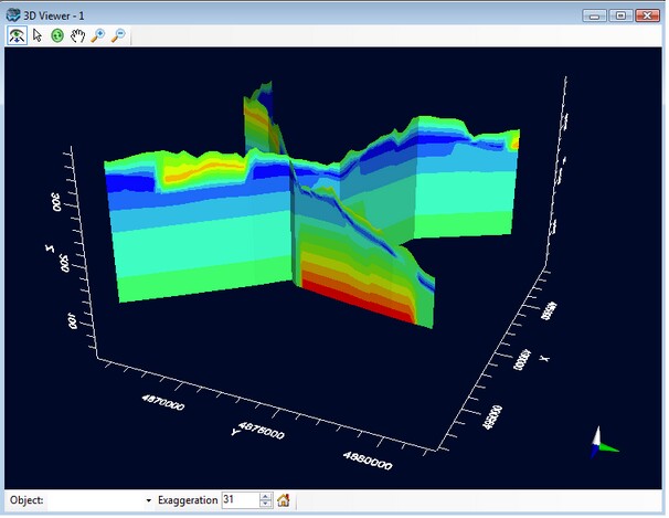
Click Apply and the display will update with the appropriate cross-section lines. An example for two cross-sections is shown below.

In the Settings tree, under Colormap -- Colors, you can access the color page where you can choose which attribute you want to render; in the case of Properties (or Recharge and Evapotranspiration) you can render by Zone or by the specified Attribute (eg. Kx, Recharge rate, etc..). For more information on the color by attribute feature, please refer to "Color By Attribute" section.

Isolines

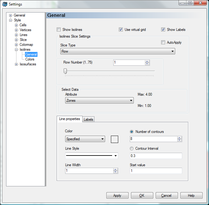
Settings for the Isolines are identical to those explained above for Slice.

Isolines also has an option to plot on a Cross-Section; see Colormap on Cross Section as described above.

Under Select Data, choose the attribute you want to use for calculating Isolines: For Properties, you can choose from Zones or Attributes (eg. Kx).

Additional Settings for Line Properties allow you to adjust the Line color, style, width. And, the number of contour lines, or the contour interval, and the starting value (minimum) by which contour intervals will be calculated. Settings in the Labels tab allow you to adjust the font size and color and the decimal format.

In the Settings tree, under Isolines -- Colors, you can access the color page where you can choose which attribute you want to render; in the case of Properties (or Recharge and Evapotranspiration) you can render by Zone or by the specified Attribute (eg. Kx, Recharge rate, etc..). For more information on the color by attribute feature, please refer to "Color By Attribute" section.

Isosurfaces

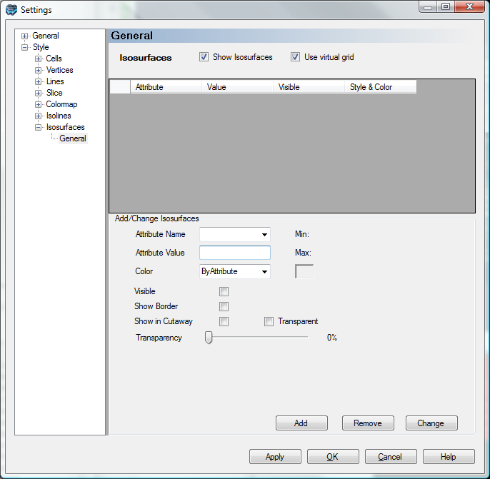
The IsoSurface node allow you to create and modify one or more isosurfaces from 3D gridded attribute data. An isosurface is a 3D planar surface defined by a constant parameter value in 3D space. Isosurfaces are typically used for demonstrating the spatial distribution of a selected parameter. For groundwater modeling purposes, isosurfaces are generally used for representing the spatial distribution of heads, drawdowns and concentrations.

Creating an Isosurface

To create an isosurface, follow the steps below:

·	From the Attribute Name combo box, select the attribute from which the isosurface is to be created.

·	Specify the attribute value in the Attribute Value field.

·	Select the color method from the Color box. The isosurface can be displayed as a solid color (Custom) or rendered by a specified attribute (ByAttribute).

·	Use the Visible check box to show/hide the isosurface.

·	Use the Show Border check box to display/hide a color map of the element value on the borders (sides) of the model domain when the isosurface intersects the edge of the model domain.

·	Use the Show in Cutaway check box to make the isosurface visible/invisible in cutaways.

·	Use the transparent check box to enable/disable transparency. If enabled, use the Transparency slider to set the level of transparency/opaqueness.

·	Click the [Add] button to create the isosurface.

The isosurface will be added to the isosurface table.

Modifying an Isosurface

To modify an existing isosurface, follow the steps below:

·	Select the isosurface from the isosurface table.

·	Make the modifications to the desired settings, e.g., attribute name, attribute value, color, etc.

·	Click the [Change] button to apply the changes.

Time

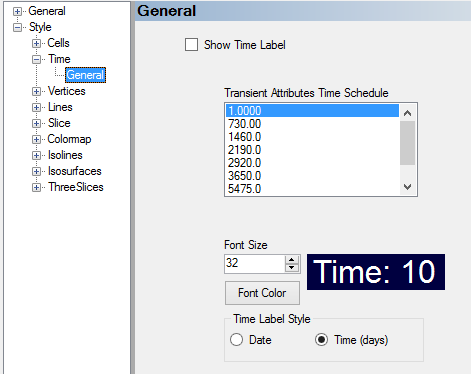
The Time node provides a list of all the time steps in the 3D gridded data object, and allows you to select the desired time step data to display in the 3D Viewer window. For 3D gridded data objects generated by steady state flow models, only one time step will be available. For 3D gridded data objects generated by transient flow models, multiple time steps will be available (as defined in the Translation settings in VMOD Flex, i.e, Translation / Time Steps).

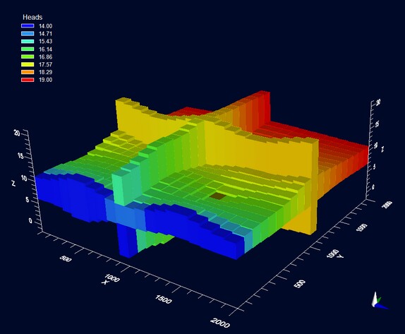
ThreeSlices

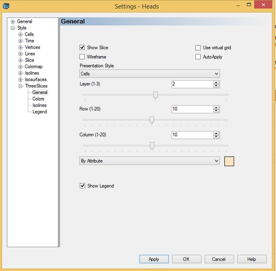
The ThreeSlices option allows you to see a slice through a selected model layer, row, and column at the same time in the 3D view. This is the display option that is used when you view 3D Gridded objects in the 3D View of the Flex Viewer. An example is shown below, with a slice through layer 2, and the centermost row and column in the Airport Transport tutorial project.

The generic options for "Slice" apply to the ThreeSlice including the Wireframe and "Use virtual grid" option.

The Colors and Legend options under ThreeSlice are also the same as described in earlier sections for Slice

The following options are unique to ThreeSlice:

·	Presentation Style: Choose between Cells and Surface; when Surface is selected, you will see a color map with Isolines; under the Isoline node in the Settings tree, you can adjust the contour interval and line style.

·	Below Presentation Style, select the desired Layer, Row, and Column number for the slice.