Navigation:  MODFLOW-2000/2005 Numerical Modeling Workflow > Define Numerical Model

 

The next step is to choose to Import Model (import VMOD Classic project or MODFLOW files), or Create Grid (create an empty grid).

 

 

 

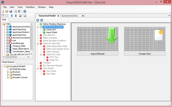
Import Model

 

You can import a Visual MODFLOW project or a USGS MODFLOW 2000/2005 data set.

 

 

 

 

When you click on the Import Model button, the following dialog will appear:

 

 

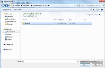
To import your Visual MODFLOW project, select the .VMF file and click Open to continue.

To import a MODFLOW data set, change the file type to "MODFLOW 2000 or MODFLOW 2005", then select the desired .NAM file,and click Open to continue.

 

Once the model is finished importing, click (Next Step) to proceed.

 

Create Grid

If you select the Create Grid option, the following window will appear.

 

 

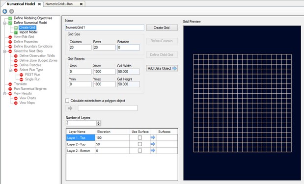
At this step, you can define the Horizontal Grid (grid size and the extents), and the Vertical Grid (number of layers and the layer elevations).

 

Define Horizontal Grid

Define the Grid size (number of Columns and Rows), Rotation, and the Grid Extents.

 

There is no limit on the grid size you can use, however if you design a grid that exceeds approximately 500,000 cells, it is strongly recommended that you use the 64-bit version, as more memory will be required to accommodate these model sizes.  (With the 64-bit version of VMOD Flex, running on 64-bit Windows and having at least 10 GB RAM, you should be able to create grids in excess of 5 million cells).

 

The grid extents can be defined manually; enter the min and max values for the X and Y co-ordinates.

 

Alternatively, the extents can be calculated from a bounding polygon.  Select the option "Calculate extents from a polygon object". You will need to import a polygon object (from .SHP or .DXF File), that contains just a single, closed polygon, and provide this is as an input.  For details on importing polygon objects, see the section Import Polygons.  Once the polygon is imported, it will appear in the Data tree in the top left.  Select/click on this polygon from the Data tree, then click on the blue arrow button under "Calculate extents from a polygon". The polygon should appear, and the X and Y extents will be calculated accordingly. (note VMOD Flex will calculate a minimum bounding rectangle from an irregularly-shaped polygon, in order to calculate the X and Y min/max extents.

 

Define Vertical Grid

 

Specify the number of layers you want for the grid.  In the table below, you can manually define a constant (flat) layer elevation for the top of each layer, and the bottom of the bottommost layer (by default, VMOD Flex will calculate equally thick layers)

 

At this step, you can also defined varying layer elevations by using surfaces. This is intended for "simple" numerical models where there are "pancake-layer geology". If your model has layers that pinchouts and/or discontinuities, it is advised that you follow the Conceptual Model workflow, as this will allow you to better accommodate more complex geology, using Horizon rules.

 

To define Surfaces for Grid layers, first you need to Create Surfaces (import then interpolate XYZ points) or Import Surfaces (from Surfer .GRD, ESRI .ASC, etc.).  Once the surfaces are available in the Data tree, select each surface for the appropriate layer elevation, being sure to work your way downwards (define top of layer 1 first, then work downwards).

 

 

 

 

Once you are finished defining the horizontal and vertical grid, click on the [Create Grid] button at the top (middle) of the window.

 

Once the grid is created, there are several options to customize the grid to your project needs.
 

The Refine/Coarsen button will load a window where you can refine/coarsen the grid. For more details on this option, please see the Edit Grid section.

 

The Define Child Grid button will load a window where you can create child (local) grids for a MODFLOW-LGR run. For more details, please see the .Define Child Grid (for LGR) section.

 

When you are finished with the grid edits, click on the (Next Step) to proceed.  This will generate the model tree structure (in the lower left corner of the window), with Inputs and Outputs.